How to visualize the intermediate layers of a network in PyTorch?

Visualizing intermediate layers of a neural network in PyTorch can help understand how the network processes input data at different stages. Visualizing intermediate layers helps us see how data changes as it moves through a neural network. We can understand what features the network learns and how they change in each layer. This helps find problems in the model, like vanishing gradients or overfitting and makes it easier to improve the model’s performance.

Need to Visualize Intermediate Layers of a Network in PyTorch

In PyTorch, the intermediate layers of a neural network serve several critical purposes. Firstly, they play a key role in feature extraction by transforming raw input data into higher-level representations, capturing relevant features essential for the given task. Additionally, visualizing activations from these layers aids in comprehending the network’s learning process at different stages, offering valuable insights into its internal mechanisms. Moreover, in transfer learning, leveraging intermediate layers from pre-trained models enables fine-tuning on new tasks while retaining previously learned knowledge. Lastly, examining intermediate activations serves as a powerful tool for debugging, facilitating the identification and resolution of issues such as vanishing or exploding gradients, as well as ineffective feature learning strategies.

Visualizing the Intermediate Layers of Network in PyTorch

PyTorch makes it easy to build neural networks and access intermediate layers. By using PyTorch’s hooks, we can intercept the output of each layer as data flows through the network. This help us extract and visualize intermediate activations, helping us understand how the network learns and processes information. To visualization the intermediate layers of a neural network in PyTorch, we will follow these steps:

Step 1: Define the Neural Network

Create a convolutional neural network with three convolutional layers and max-pooling using PyTorch’s nn.Module class. Then make an instance of the network.

• A simple neural network is defined using the MyNetwork class, which inherits from nn.Module.
• It consists of three convolutional layers (conv1, conv2, conv3), each followed by a ReLU activation function, and max-pooling layers (pool).

Python3

import torch
import torch.nn as nn

# Define your neural network
class MyNetwork(nn.Module):
    def __init__(self):
        super(MyNetwork, self).__init__()
        self.conv1 = nn.Conv2d(3, 16, kernel_size=3, stride=1, padding=1)
        self.conv2 = nn.Conv2d(16, 32, kernel_size=3, stride=1, padding=1)
        self.conv3 = nn.Conv2d(32, 64, kernel_size=3, stride=1, padding=1)
        self.pool = nn.MaxPool2d(2, 2)
        self.relu = nn.ReLU()

    def forward(self, x):
        x = self.relu(self.conv1(x))
        x = self.pool(x)
        x = self.relu(self.conv2(x))
        x = self.pool(x)
        x = self.relu(self.conv3(x))
        x = self.pool(x)
        return x

# Instantiate your network
net = MyNetwork()

Step 2: Register Forward Hooks

Next, create a hook function to collect the intermediate activations of specific layers during the forward pass. Register the hook functions for the desired intermediate layers of the network.

• A hook function get_activation is defined, which takes the name of the layer as input.
• This function returns another function, which is the actual hook. This hook is called during the forward pass and collects the activations of the layer specified by the name.

Python3

# Define a hook function to collect intermediate activations
activations = {}
def get_activation(name):
    def hook(model, input, output):
        activations[name] = output.detach()
    return hook

# Register hooks for intermediate layers
net.conv1.register_forward_hook(get_activation('conv1'))
net.conv2.register_forward_hook(get_activation('conv2'))
net.conv3.register_forward_hook(get_activation('conv3'))

Step 3: Forward Pass and Collect Activations

Now, create a sample input tensor. Perform a forward pass through the network while collecting the intermediate activations using the registered hooks.

• Hooks are registered for the intermediate convolutional layers (conv1, conv2, conv3).
• These hooks will call the get_activation function, collecting the activations of the corresponding layers during forward passes.

Python3

# Create a sample input
input_tensor = torch.randn(1, 3, 32, 32)

# Forward pass with hooks
output = net(input_tensor)

Step 4: Visualize Intermediate Activations

Now, Iterate through the collected activations, printing their shapes, and displaying them as grayscale images using Matplotlib. Each image represents the activations of a single feature map in the corresponding layer of the neural network.

• The collected activations are visualized using Matplotlib.
• For each intermediate layer, the shape of the activation tensor is printed, and a grayscale image of the first channel of the activation tensor is displayed.
• The title of each subplot indicates the layer name.

Python3

import matplotlib.pyplot as plt

# Visualize the intermediate activations
for layer_name, activation in activations.items():
    print(f'Layer: {layer_name}, Shape: {activation.shape}')
    plt.imshow(activation[0, 0].cpu().numpy(), cmap='gray')
    plt.title(layer_name)
    plt.show()

Output:

Layer: conv1, Shape: torch.Size([1, 16, 32, 32])
Layer: conv2, Shape: torch.Size([1, 32, 16, 16])
Layer: conv3, Shape: torch.Size([1, 64, 8, 8])

For the first convolutional layer (conv1), the shape of the output activation is [1, 16, 32, 32], indicating 16 channels with a spatial dimension of 32×32.

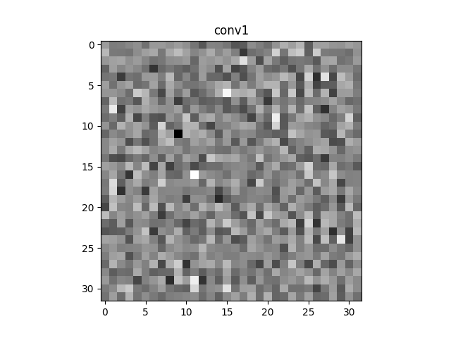
Layer: conv1

• Shape: torch.Size([1, 16, 32, 32])
• This indicates that the output of the first convolutional layer (conv1) has a shape of (1, 16, 32, 32).
• Here, 1 represents the batch size (one image processed), 16 represents the number of output channels or feature maps generated by the convolution operation.
• The dimensions 32×32 represent the spatial dimensions of the feature maps. Each feature map has a size of 32×32.

Visualization

• A grayscale image is displayed, representing the activations of the first channel of the conv1 layer. Each pixel in this image corresponds to the activation value of a particular neuron in the feature map.
• The image visually depicts the features learned by the conv1 layer for the given input image.

For the second convolutional layer (conv2), the shape of the output activation is [1, 32, 16, 16], showing 32 channels with a spatial dimension of 16×16.

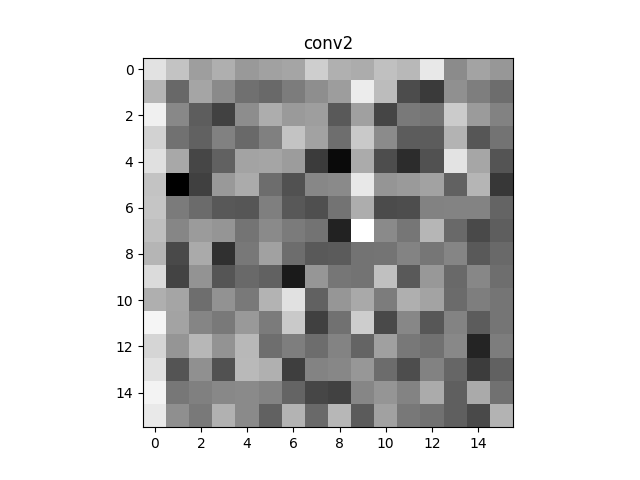
Layer: conv2

• Shape: torch.Size([1, 32, 16, 16])
• The output of the second convolutional layer (conv2) has a shape of (1, 32, 16, 16).
• Similar to conv1, 1 represents the batch size, but now we have 32 channels or feature maps.
• The spatial dimensions are reduced to 16×16, indicating that the features are further abstracted and downsampled compared to the output of conv1.

Visualization

• Another grayscale image is displayed, representing the activations of the first channel of the conv2 layer.
• The image illustrates the learned features at a deeper layer in the network, showing how the input is transformed through successive layers.

For the third convolutional layer (conv3), the shape of the output activation is [1, 64, 8, 8], revealing 64 channels with a spatial dimension of 8×8.

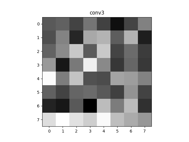
Layer: conv3

• Shape: torch.Size([1, 64, 8, 8])
• The output of the third convolutional layer (conv3) has a shape of (1, 64, 8, 8).
• Again 1 represents the batch size, and now we have 64 channels or feature maps.
• The spatial dimensions are further reduced to 8×8, indicating more abstract and high-level features.

Visualization

• A third grayscale image is displayed, representing the activations of the first channel of the conv3 layer.
• This image demonstrates the most abstract and high-level features learned by the network, as it’s closer to the output and captures complex patterns in the input image.