How to visualize training progress in PyTorch?

Deep learning and understanding the mechanics of learning and progress during training is vital to optimize performance while diagnosing problems such as underfitting or overfitting. The process of visualizing training progress offers valuable insights into the dynamics of learning that allow us to make sound decisions. In this article, we will learn how to visualize the training progress in Pytorch.

Two methods by which training progress must be visualized are:

• Using Matplotlib
• Using Tensor Board

Visualizing Training Progress in PyTorch Using Matplotlib

Matplotlib is a widely used plotting library in Python that provides a flexible and powerful tool for creating static, animated, and interactive visualizations in Python. It is particularly well-suited for creating publication-quality plots and charts.

Step 1: Import Necessary Libraries and Generate a Sample Dataset

In this step, we are going to import necessary libraries and generate sample dataset.

import torch
import torch.nn as nn
import torch.optim as optim
import matplotlib.pyplot as plt
# Sample data
X = torch.randn(100, 1)  # Sample features
y = 3 * X + 2 + torch.randn(100, 1)  # Sample labels with noise

Step 2: Define the Model

1. The `LinearRegression` class in PyTorch defines a simple linear regression model. It inherits from the `nn.Module` class, making it a neural network model.
2. The constructor (`__init__` method) initializes the model’s structure, creating a single linear layer (`nn.Linear`) with one input feature and one output feature.
3. This linear layer is stored as an attribute named `self.linear`. The `forward` method defines how input data `x` is processed through this linear layer to produce the model’s output.
4. Specifically, the input `x` is passed through `self.linear`, and the resulting output is returned. This method encapsulates the forward pass computation of the neural network, determining how inputs are transformed into outputs by the model.

# Define a simple linear regression model
class LinearRegression(nn.Module):
    def __init__(self):
        super(LinearRegression, self).__init__()
        self.linear = nn.Linear(1, 1)  # One input feature, one output

    def forward(self, x):
        return self.linear(x)

model = LinearRegression()

Step 3: Define the Loss Function, Optimizer and Training Loop

In the following code, we have define Mean Squared Error as the loss function and Stochastic Gradient Descent(SGD) optimizer as optimizer that modifies the model’s parameters by using calculated gradients with a learning rate of 0.01.

# Define loss function and optimizer
criterion = nn.MSELoss()
optimizer = optim.SGD(model.parameters(), lr=0.01)

This code runs a training loop for a neural network model over multiple epochs, computing and optimizing the loss using gradient descent. Loss values are stored for plotting, and progress is printed every 10 epochs.

# Training loop
num_epochs = 100
losses = []
for epoch in range(num_epochs):
    # Forward pass
    outputs = model(X)
    loss = criterion(outputs, y)

    # Backward pass and optimization
    optimizer.zero_grad()
    loss.backward()
    optimizer.step()

    # Print progress
    if (epoch+1) % 10 == 0:
        print(f'Epoch [{epoch+1}/{num_epochs}], Loss: {loss.item():.4f}')

    # Store loss for plotting
    losses.append(loss.item())

Step 4: Visualizing Training Progress in PyTorch using Matplotlib

Using the following code, we can visualize the training loss curve using matplotlib.

• The plt.plot(losses) line plots the loss values stored in the losses list against the epoch number.
• The x-axis represents the epoch number, and the y-axis represents the corresponding loss value.
• The plt.xlabel(‘Epoch’), plt.ylabel(‘Loss’), and plt.title(‘Training Loss’) lines set the labels and title for the plot.
• Finally, plt.show() displays the plot, allowing you to visually analyze how the loss decreases (or converges) over the training epochs.

# Plot the loss curve
plt.plot(losses)
plt.xlabel('Epoch')
plt.ylabel('Loss')
plt.title('Training Loss')
plt.show()

Typically, you would expect to see a decreasing trend in the loss curve, indicating that the model is learning and improving over time.

Complete Code:

Python3

import torch
import torch.nn as nn
import torch.optim as optim
import matplotlib.pyplot as plt

# Sample data
X = torch.randn(100, 1)  # Sample features
y = 3 * X + 2 + torch.randn(100, 1)  # Sample labels with noise

# Define a simple linear regression model
class LinearRegression(nn.Module):
    def __init__(self):
        super(LinearRegression, self).__init__()
        self.linear = nn.Linear(1, 1)  # One input feature, one output

    def forward(self, x):
        return self.linear(x)

model = LinearRegression()

# Define loss function and optimizer
criterion = nn.MSELoss()
optimizer = optim.SGD(model.parameters(), lr=0.01)

# Training loop
num_epochs = 100
losses = []
for epoch in range(num_epochs):
    # Forward pass
    outputs = model(X)
    loss = criterion(outputs, y)

    # Backward pass and optimization
    optimizer.zero_grad()
    loss.backward()
    optimizer.step()

    # Print progress
    if (epoch+1) % 10 == 0:
        print(f'Epoch [{epoch+1}/{num_epochs}], Loss: {loss.item():.4f}')

    # Store loss for plotting
    losses.append(loss.item())
    
# Plot the loss curve
plt.plot(losses)
plt.xlabel('Epoch')
plt.ylabel('Loss')
plt.title('Training Loss')
plt.show()
   

Output:

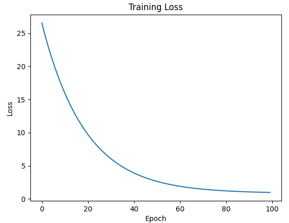
Visualizing loss at each epoch using matplotlib.

The output graph shows how the training loss changes with time as plotted against number of iterations. This visualization enables one to see how a model reduces its loss when being trained. Further, the Matplotlib plot have other things like axes labels, titles and maybe markers or lines indicating specific events such as minimum achieved loss or sharp declines in losses.

Visualizing Training Progress Using TensorBoard

In order to visualize the training process in a deep learning model, we can use SummaryWriter class from torch.utils.tensorboard module, which seamlessly integrates with TensorBoard, a visualization tool developed by TensorFlow.

• Integration: PyTorch provides a SummaryWriter class in the torch.utils.tensorboard module, which integrates seamlessly with TensorBoard for visualization.
• Logging: Inside the training loop, you can use SummaryWriter to log various metrics like loss, accuracy, etc., for visualization.
• Visualization: TensorBoard provides interactive and real-time visualizations of the logged metrics, allowing you to monitor the training progress dynamically.
• Monitoring: TensorBoard enables you to monitor multiple aspects of training, such as learning curves, model graphs, and histogram of weights, providing insights for optimizing your model.

Install the TensorBoard library using the following command:

pip install tensorboard

Step 1: Import Libraries

import torch
import torch.nn as nn
import torch.optim as optim
import torchvision
import torchvision.transforms as transforms
from torch.utils.data import DataLoader
from torch.utils.tensorboard import SummaryWriter

Step 2: Define a Simple Neural Network

Lets define SimpleNN a class declaration of a simple neural network containing two layers that are fully connected, along with forward function that defines the forward pass of the network.

# Define a simple neural network
class SimpleNN(nn.Module):
    def __init__(self):
        super(SimpleNN, self).__init__()
        self.fc1 = nn.Linear(784, 128)
        self.fc2 = nn.Linear(128, 10)

    def forward(self, x):
        x = torch.flatten(x, 1)
        x = torch.relu(self.fc1(x))
        x = self.fc2(x)
        return x

Step 3: Load MNIST Dataset

Let us load the MINST data for training, divide it into batches and apply transformation by using some preprocessing techniques.

# Load a smaller subset of MNIST dataset
transform = transforms.Compose([
    transforms.ToTensor(),
    transforms.Normalize((0.5,), (0.5,))
])

train_dataset = torchvision.datasets.MNIST(root='./data', train=True, transform=transform, download=True)
small_train_dataset = torch.utils.data.Subset(train_dataset, range(1000))  # Subset of first 1000 samples
train_loader = DataLoader(small_train_dataset, batch_size=64, shuffle=True)

Step 4: Initialize Model, Loss Function, and Optimizer

Now, initialize model. Along with it we will be using cross-entropy loss function and adam optimizer for updating model parameters.

# Initialize model, loss function, and optimizer
model = SimpleNN()
criterion = nn.CrossEntropyLoss()
optimizer = optim.Adam(model.parameters(), lr=0.001)

Step 5: Initialize SummaryWriter for Logging

SummaryWriter is object of imported module to write logs to be visualized in TensorBoard.

# Initialize SummaryWriter for logging
writer = SummaryWriter('logs_small')

Step 6: Training Loop

• Training Loop: Goes through the epochs and batches, performs forward pass, computes loss, backward pass and updates model parameters.
• Log Loss and Accuracy: The epoch-wise training loss and accuracy are being logged.

# Training loop
epochs = 5
for epoch in range(epochs):
    running_loss = 0.0
    correct = 0
    total = 0

    for i, (inputs, labels) in enumerate(train_loader):
        optimizer.zero_grad()
        outputs = model(inputs)
        loss = criterion(outputs, labels)
        loss.backward()
        optimizer.step()

        running_loss += loss.item()

        # Calculate accuracy
        _, predicted = torch.max(outputs, 1)
        total += labels.size(0)
        correct += (predicted == labels).sum().item()

        # Log loss
        writer.add_scalar('Loss/train', loss.item(), epoch * len(train_loader) + i)

    # Log accuracy
    accuracy = 100 * correct / total
    writer.add_scalar('Accuracy/train', accuracy, epoch)

    print(f'Epoch [{epoch+1}/{epochs}], Loss: {running_loss / len(train_loader)}, Accuracy: {accuracy}%')

print('Finished Training')
writer.close()

Complete Code:

Python3

import torch
import torch.nn as nn
import torch.optim as optim
import torchvision
import torchvision.transforms as transforms
from torch.utils.data import DataLoader
from torch.utils.tensorboard import SummaryWriter

# Define a simple neural network
class SimpleNN(nn.Module):
    def __init__(self):
        super(SimpleNN, self).__init__()
        self.fc1 = nn.Linear(784, 128)
        self.fc2 = nn.Linear(128, 10)

    def forward(self, x):
        x = torch.flatten(x, 1)
        x = torch.relu(self.fc1(x))
        x = self.fc2(x)
        return x
      
# Load a smaller subset of MNIST dataset
transform = transforms.Compose([
    transforms.ToTensor(),
    transforms.Normalize((0.5,), (0.5,))
])

train_dataset = torchvision.datasets.MNIST(root='./data', train=True, transform=transform, download=True)
small_train_dataset = torch.utils.data.Subset(train_dataset, range(1000))  # Subset of first 1000 samples
train_loader = DataLoader(small_train_dataset, batch_size=64, shuffle=True)

# Initialize model, loss function, and optimizer
model = SimpleNN()
criterion = nn.CrossEntropyLoss()
optimizer = optim.Adam(model.parameters(), lr=0.001)

# Initialize SummaryWriter for logging
writer = SummaryWriter('logs_small')


# Training loop
epochs = 5
for epoch in range(epochs):
    running_loss = 0.0
    correct = 0
    total = 0

    for i, (inputs, labels) in enumerate(train_loader):
        optimizer.zero_grad()
        outputs = model(inputs)
        loss = criterion(outputs, labels)
        loss.backward()
        optimizer.step()

        running_loss += loss.item()

        # Calculate accuracy
        _, predicted = torch.max(outputs, 1)
        total += labels.size(0)
        correct += (predicted == labels).sum().item()

        # Log loss
        writer.add_scalar('Loss/train', loss.item(), epoch * len(train_loader) + i)

    # Log accuracy
    accuracy = 100 * correct / total
    writer.add_scalar('Accuracy/train', accuracy, epoch)

    print(f'Epoch [{epoch+1}/{epochs}], Loss: {running_loss / len(train_loader)}, Accuracy: {accuracy}%')

print('Finished Training')
writer.close()

Output:

Epoch [1/5], Loss: 1.9477481991052628, Accuracy: 37.9%
Epoch [2/5], Loss: 1.207241453230381, Accuracy: 73.4%
Epoch [3/5], Loss: 0.8120987266302109, Accuracy: 80.9%
Epoch [4/5], Loss: 0.6294657941907644, Accuracy: 84.7%
Epoch [5/5], Loss: 0.5223450381308794, Accuracy: 86.5%
Finished Training

Visualizing Training Progress in PyTorch

In order to run TensorBoard, you should open a terminal and go to the folder in which you keep your logs (stored in previous step); then to run tensorboard use command:

tensorboard --logdir=logs

Output:

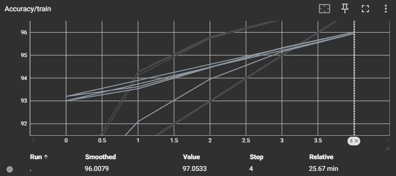
Visualizing accuracy During training.

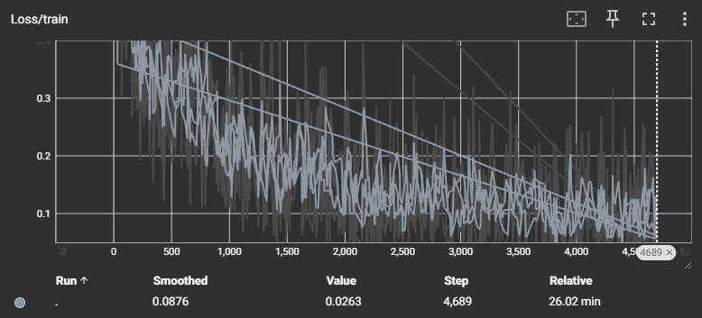
Loss during training at each step.

Accessing TensorBoard requires : Opening a browser and enter into the web address given by TensorBoard (normally http://localhost:6006/).

TensorBoard provides a web-based dashboard with tabs and visualizations representing various training aspects. Scalar metrics visualize values like loss or accuracy over epochs, offering different perspectives on training dynamics. Additionally, TensorBoard can display histograms, embeddings, and specialized visualizations based on logged information.

In this blog, we have covered how can we visualize training progress for deep learning framework using matplotlib and tensorboard.