How to Form Graphs in Tensorflow?

Tensorflow, a Google open-source machine learning toolkit, is widely used for developing and training various deep learning models. TensorFlow’s key idea is the creation of computation graphs, which specify the operations and relationships between tensors. In this article, we’ll look at how to create graphs with TensorFlow, breaking it down into simple steps with examples.

Form Graphs in Tensorflow

TensorFlow computations are represented as directed acyclic graphs (DAGs), with nodes representing operations and edges depicting data flow between these actions. This graph-based technique enables optimization during model training.

Prerequisites:

• TensorFlow

We are going to use the TensorFlow so make sure you have installed the TensorFlow into your system. If not, then use the following command to install.

! pip install tensorflow

TensorFlow

In this example, we perform basic operations using TensorFlow, adding x and y, and then multiplying the result by 2. Now, let’s add a feature to visualize the computation graph using TensorBoard. We create a directory named “logs” to store the TensorBoard logs. Then, we set up a summary writer with TensorFlow to write the logs into the specified directory. We create two TensorFlow constant tensors, x and y, with values 3 and 5, respectively. These will serve as inputs to our function. To trace the computation graph, we use tf.summary.trace_on and pass graph=True. This tells TensorFlow to trace the operations in the function and record the computation graph. Next, we call our function calculate_result with the input tensors x and y. This invocation creates and executes the computation graph. After that, we use tf.summary.trace_export to save the traced computation graph. We provide a name (“result_trace”), a step value (0 in this case), and the directory where the profiler data will be stored (which is our “logs” directory). Finally, we print the result of the computation, which is the output tensor obtained from our function.

Python3

import tensorflow as tf

@tf.function
def calculate_result(x, y):
    result = tf.add(x, y)
    result = tf.multiply(result, 2)
    return result

log_dir = "logs/"
writer = tf.summary.create_file_writer(log_dir)

x = tf.constant(3)
y = tf.constant(5)

tf.summary.trace_on(graph=True, profiler=False)
output = calculate_result(x, y)

with writer.as_default():
    tf.summary.trace_export(name="result_trace", step=0, profiler_outdir=log_dir)

print("Result:", output.numpy())

Save the above code as Name.py

To run the python code, Open the terminal use the following command:

python script_name.py  #  Replace the script_name.py with the path of save python file

Output:

16

When we run the code, it will create a folder named “logs”. It is the summary logs, Which is stored in this ‘logs’ directory.

Plot the Computation Graph

When you will run the script the summary logs will be stored in this directory. TensorBoard reads these logs and provides interactive visualizations. To visualize the graph using TensorBoard use the following command:

tensorboard --logdir logs/

and click on GRAPHS.

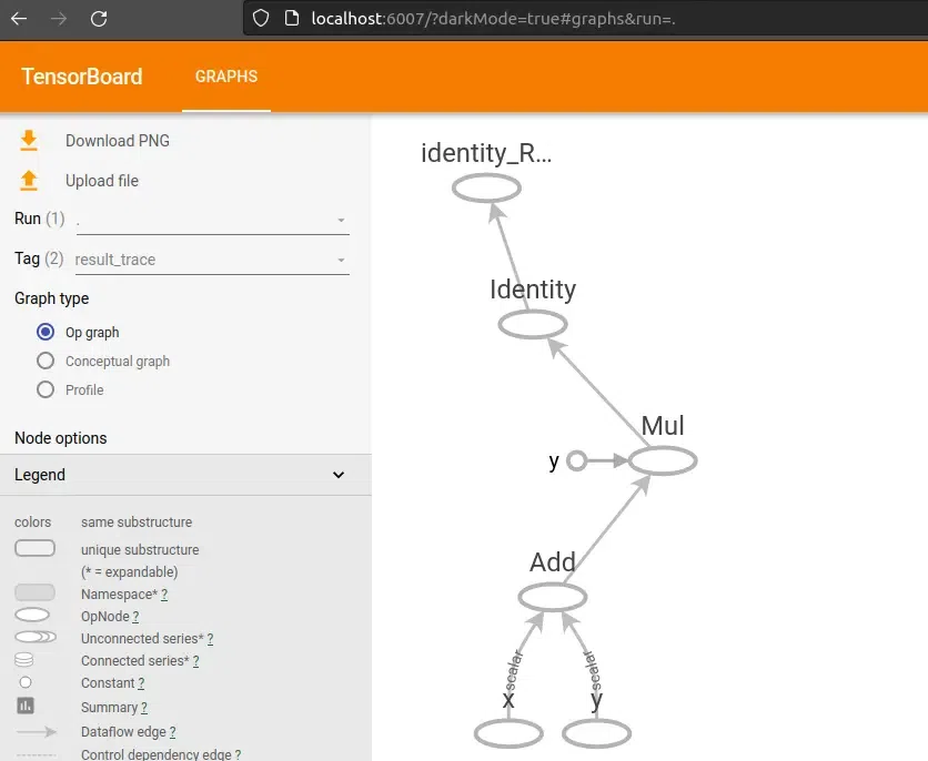
Computation Graph

Tensorflow Graph 2

In this example, we use the tf.function decorator to create a TensorFlow function that performs a simple linear transformation—specifically, the equation y = wx + b. The function accepts a tensor as input, a weight variable, and a bias variable. The weight is multiplied by the input tensor, and the bias is applied to the result. We use TensorBoard to visualize this operation by tracing the graph and saving it using tf.summary.trace_export. The input tensor is a fixed array, whereas the weight and bias are variables that can be trained.

Python3

import tensorflow as tf

@tf.function
def linear_transformation(input_tensor, weight, bias):
    result = tf.add(tf.multiply(input_tensor, weight), bias)
    return result

log_dir = "logs/"
summary_writer = tf.summary.create_file_writer(log_dir)

input_data = tf.constant([1.0, 2.0, 3.0, 4.0], name="input_data")
weight = tf.Variable(2.0, name="weight", trainable=True)
bias = tf.Variable(1.0, name="bias", trainable=True)

tf.summary.trace_on(graph=True, profiler=False)

output_tensor = linear_transformation(input_data, weight, bias)

with summary_writer.as_default():
    tf.summary.trace_export(
        name="linear_transformation_trace", step=0, profiler_outdir=log_dir
    )

print(output_tensor.numpy())

Save the above code as Name.py

To run the python code, Open the terminal use the following command:

python script_name.py # Replace the script_name.py with the path of save python file

Output:

[3. 5. 7. 9.]

When we run the code, it will create a folder named “logs”. It is the summary logs, Which is stored in this ‘logs’ directory.

Plot the Computation Graph

When you will run the script the summary logs will be stored in this directory. TensorBoard reads these logs and provides interactive visualizations. To visualize the graph using TensorBoard use the following command:

tensorboard --logdir logs/

and click on GRAPHS.

we can visualize the different different Computation Graph whose summary are stored in same lags by changing the tags.

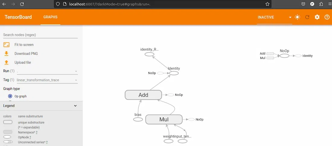
Computation Graph