How scientific mode works in PyCharm?

Over the years, Python has developed its reputation as a tool for information science that takes a great deal of mathematics, computer learning, and specific research This trend can be said if simple Python and libraries like NumPy and scikit-learn there is, designed for statistical analysis. There are also plotting libraries such as Matplotlib that mimic the interface of the MATLAB plotting function, making the switch very easy.

With a good library, and a sophisticated IDE that can guide things like graphing and monitoring variables in the program. These features are delivered through the popular Python IDE, PyCharm. This put up will be on the factors PyCharm affords and how to use it.

PyCharm Scientific Mode

PyCharm’s scientific approach bears some similarities to MATLAB, so making the switch should be comfortable for users with prior experience. Let’s jump into how to get started with PyCharm scientific prescriptions.

Step 1: Installation

The first step is to download PyCharm from the official website and install it.

Step 2: Create Scientific Mode Project

After that, run and click “Create New Project” to start the process; Click on “scientific mode”, set up your project interpreter, and click on “Create” to create your project. You should now have a window like the image below.

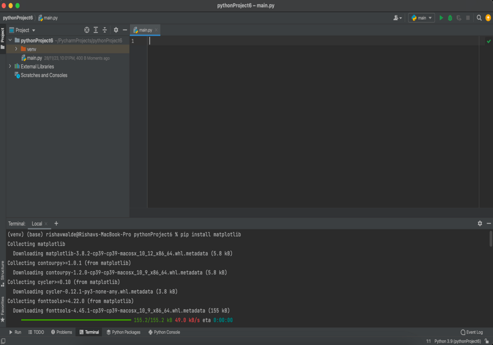
pip Install matplotlib

Step 3: Select ScieView

On the far right you will see a screen with ScieView, R Packages, R Graphics, and Database. SciView allows you to view your plots and data points right in the IDE window. This eliminates the need to switch between windows to view plots, simplifying the plot analysis task. R Packages and R Graphics are useful if you have a set of R interpreters.

There is also a window at the bottom right of the screen that shows you the changes to the last program you made, which is useful for research. If no program is running, the window displays Special Variables (which are embedded Python variables). Click on the arrow below.

Step 4: Write Simple Code

Now, let’s create a simple program and watch PyCharm’s scientific approach work. Copy and paste the code below into PyCharm and click the Run button.

Python3

import matplotlib.pyplot as plt
from mpl_toolkits.mplot3d import Axes3D
import numpy as np

def plot_torus():
    # Create a figure and 3D axis
    fig = plt.figure()
    ax = fig.add_subplot(111, projection='3d')

    # Define parameters for the torus
    major_radius = 10
    minor_radius = 3
    u = np.linspace(0, 2 * np.pi, 100)
    v = np.linspace(0, 2 * np.pi, 100)

    # Parametric equation of a torus
    u, v = np.meshgrid(u, v)
    x = (major_radius + minor_radius * np.cos(v)) * np.cos(u)
    y = (major_radius + minor_radius * np.cos(v)) * np.sin(u)
    z = minor_radius * np.sin(v)

    # Create a surface plot of the torus
    ax.plot_surface(x, y, z, cmap='viridis')

    # Set labels for the axes
    ax.set_xlabel('X-axis')
    ax.set_ylabel('Y-axis')
    ax.set_zlabel('Z-axis')

    # Set title for the plot
    ax.set_title('3D Plot of a Torus')

    # Display the plot
    plt.show()

# Call the function to execute the plot
plot_torus()

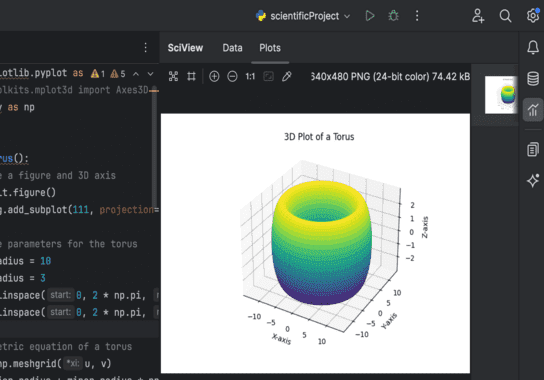
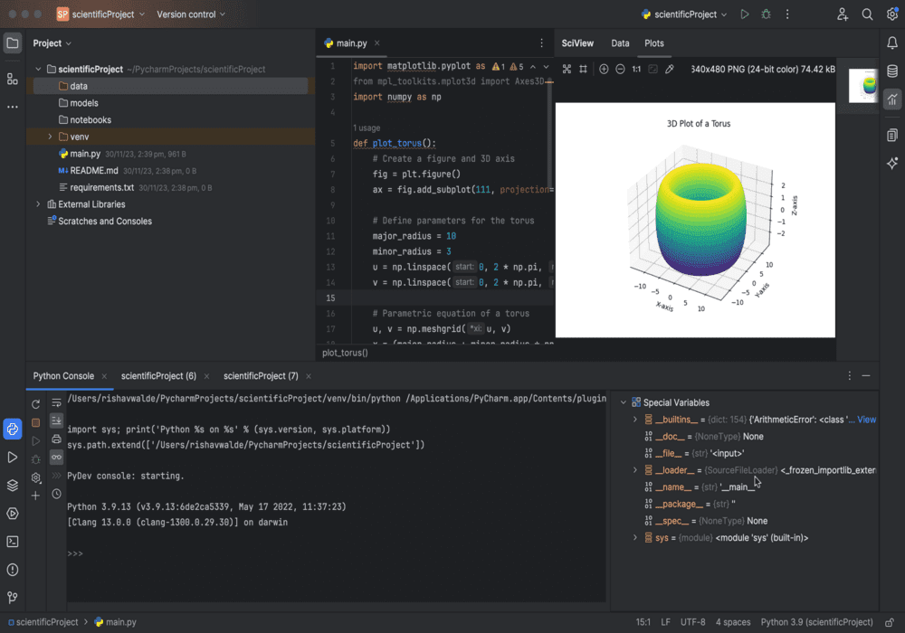
Output:

Once you run the code you should see the plot in the SciView window, the variables in the scope of the program now appear in the bottom right window. This feature can be useful for debugging and testing other things in the interactive console.

Summary

PyCharm Science Methods is a unique PyCharm IDE mode that provides tools to simplify your science or research workflow. This mode allows you to view plots in an IDE window, view variables in the last run program, and provides features for use in the R programming language.