Handling Categorical Features using LightGBM

In the realm of machine learning and predictive modelling, the effective handling of categorical features is a vital task, often crucial to the success of a model. One popular and powerful tool that excels in this aspect is LightGBM. LightGBM is a gradient-boosting framework that not only delivers impressive predictive performance but also streamlines the process of dealing with categorical data. In this discussion, we will delve into the strategies and techniques for effectively managing categorical features using LightGBM, exploring how this framework leverages its unique strengths to address the challenges posed by non-numeric data, and ultimately, to enhance the quality and efficiency of machine learning models.

What is LightGBM?

LightGBM, which stands for “Light Gradient Boosting Machine,” is an open-source, distributed machine learning framework primarily designed for boosting tasks. Microsoft developed it and is known for its efficiency and speed, making it a popular choice for various machine learning and data science applications.

LightGBM is a versatile tool for regression, classification, ranking, and many other machine-learning tasks. It’s particularly well-suited for scenarios where training speed and memory efficiency are crucial, such as in large-scale datasets and production environments.

Key features and characteristics of LightGBM

• Gradient Boosting: LightGBM is based on the gradient boosting framework, which is a powerful ensemble learning technique. It builds a strong predictive model by combining the predictions of multiple weak models
• Handling Categorical Features: LightGBM has built-in support for handling categorical features. It can efficiently handle high-cardinality categorical data without requiring extensive preprocessing.
• Custom Objective and Evaluation Functions: You can define custom loss functions and evaluation metrics, which is valuable for tackling specific machine learning problems.
• GPU Acceleration: LightGBM supports GPU acceleration for even faster training and prediction.

What are categorical features?

Categorical features, also known as discrete or qualitative features, are a type of data variable in statistics and machine learning that represent categories or labels. These features typically take on a limited, fixed number of distinct values, and they do not have a natural ordering between them. Understanding and properly handling categorical features is important in data analysis and machine learning, as they require special treatment compared to continuous (numeric) features. Here are the key characteristics and details about categorical features:

• Distinct Categories: Categorical features have a finite number of unique categories or labels. Examples include colors (red, blue, green), days of the week (Monday, Tuesday, etc.), or product names.
• No Inherent Order: Categorical values do not have a natural order or ranking. In other words, you can’t say that one category is “greater” or “lesser” than another in a meaningful way.
• Encoding: Categorical features need to be encoded into numerical values before they can be used in most machine learning algorithms. Common encoding methods include one-hot encoding (creating binary columns for each category), label encoding (assigning each category a unique integer), and more advanced methods like target encoding.
• Dummy Variables: One-hot encoding is a popular method for dealing with categorical features. It transforms a categorical feature into binary (0 or 1) dummy variables for each category. This allows machine learning algorithms to treat each category separately.
• Curse of Dimensionality: When one-hot encoding is used, adding many binary columns for each category can lead to a high-dimensional dataset, which may result in increased computational complexity and potentially overfitting. Care must be taken to avoid the “curse of dimensionality.”

Handling Categorical features in LightGBM

Handling categorical features in a dataset effectively is made possible by LightGBM’s helpful feature named categorical_feature. Discrete categories, like gender, nation, or product category, are represented by variables known as categorical features. In gradient boosting machine learning models, for example, they need to be handled differently.

It is possible to designate which columns in your dataset are categorical using the categorical_feature parameter. It is LightGBM’s internal tree-building algorithms that adjust to accommodate categorical features when you define them with this parameter. Both the model’s training speed and forecast accuracy can be greatly enhanced by making this adjustment.

LightGBM prevents interpreting categorical features as continuous variables, which would result in an ineffective and subpar splitting procedure during tree construction. Instead, it identifies categorical characteristics. For accurate and efficient splits, it instead makes use of strategies like histogram-based approaches. Ultimately, when working with datasets containing categorical variables, LightGBM’s categorical_feature parameter is essential for optimizing the model’s predictive power while reducing computational resources and training time.

Implementation to Handle Categorical Features

In this code, we’ll use the famous Titanic dataset, which contains information about passengers on the Titanic, and we’ll focus on the “Sex” and “Embarked” features as categorical features. The goal is to predict whether a passenger survived or not.

First, make sure you have the lightgbm library installed. You can install it using pip if you haven’t already.

!pip install lightgbm

Importing Libraries

Python

import lightgbm as lgb
import pandas as pd
from sklearn.model_selection import train_test_split
from sklearn.metrics import accuracy_score
import matplotlib.pyplot as plt

• lightgbm for the LightGBM framework.
• pandas for data manipulation.
• train_test_split from sklearn for splitting the data into training and validation sets.
• accuracy_score from sklearn to evaluate the model’s accuracy.

Load the Titanic Dataset

We load the Titanic dataset from a URL

Python

url = "https://web.stanford.edu/class/archive/cs/cs109/cs109.1166/stuff/titanic.csv"
data = pd.read_csv(url)
print(data.head())

Output:

  Survived  Pclass                                               Name  \
0         0       3                             Mr. Owen Harris Braund   
1         1       1  Mrs. John Bradley (Florence Briggs Thayer) Cum...   
2         1       3                              Miss. Laina Heikkinen   
3         1       1        Mrs. Jacques Heath (Lily May Peel) Futrelle   
4         0       3                            Mr. William Henry Allen   
      Sex   Age  Siblings/Spouses Aboard  Parents/Children Aboard     Fare  
0    male  22.0                        1                        0   7.2500  
1  female  38.0                        1                        0  71.2833  
2  female  26.0                        0                        0   7.9250  
3  female  35.0                        1                        0  53.1000  
4    male  35.0                        0                        0   8.0500  

Using pandas, this code loads the Titanic dataset from the given URL and uses the head() function to show the first five rows of the dataset. It offers a preliminary look at the organization and content of the dataset.

Python3

# Selecting features 'Pclass', 'Age', and 'Fare' and assigning them to 'X'
X = data[['Pclass', 'Age', 'Fare']]
# Selecting the 'Survived' column as the target variable 'y'
y = data['Survived']

Here, we choose particular columns (‘Pclass,’ ‘Age,’ and ‘Fare’) from the ‘data’ DataFrame to generate a feature matrix (‘X’). For the machine learning model, these columns will serve as input features.The target variable ‘y’ is assigned the ‘Survived’ column from the ‘data’ DataFrame. To indicate whether or whether the passengers survived, this column has binary labels (0 or 1). The values that we wish our model to predict are represented by the letter “y.”

Split Data into Training and Validation Sets

We split the data into training and validation sets

Python

# Split the feature and target data into training and validation sets using a 80-20 split ratio.
X_train, X_valid, y_train, y_valid = train_test_split(
    X, y, test_size=0.2, random_state=42)

In order to evaluate the model, this code separates the data into two sets: training (X_train and y_train) and validation (X_valid and y_valid). For reproducibility, a fixed random seed (random_state) is used. For training, the split ratio is set at 80% and for validation, to 20%.

Create LightGBM Datasets

We create LightGBM datasets for training and validation.

Python

# Create LightGBM datasets for training and validation using X_train, y_train, X_valid, and y_valid.
train_data = lgb.Dataset(X_train, label=y_train, categorical_feature=['Pclass'])
valid_data = lgb.Dataset(X_valid, label=y_valid, reference=train_data)

We generate a ‘train_data’ LightGBM dataset for training purposes. It is built with the matching labels, “y_train,” and the training features, “X_train.” Furthermore, we indicate that the columns “Pclass” is the categorical characteristics. In gradient boosting models, categorical characteristics frequently need special handling.

Likewise, we generate an additional LightGBM dataset called ‘valid_data’ in order to conduct validation. The validation features “X_valid” and the matching labels “y_valid” are used in its construction. To maintain uniformity when managing categorical features, we additionally supply a reference to the ‘train_data’ dataset.

Set Model Parameters

We define the parameters for the LightGBM model.

Python

params = {
    'objective': 'binary',
    'metric': 'binary_logloss',
    'boosting_type': 'gbdt',
    'num_leaves': 11,
    'learning_rate': 0.05,
}

The provided params dictionary contains configuration settings for a LightGBM binary classification model:

• objective: “binary”: Indicates that the model’s goal is to classify binary data.
• metric: 'binary_logloss': Evaluates the model using binary log-loss as the metric.
• boosting_type: 'gbdt': Chooses the gradient boosting decision tree as the boosting type.
• num_leaves: 31: Sets the maximum number of leaves in each tree to 31.Step 9: Train the Model
• learning_rate: 0.05: Defines the learning rate for the gradient boosting process.

Training the LightGBM Model

Python

num_round = 100
bst = lgb.train(params, train_data, num_round,
                valid_sets=[train_data, valid_data])

This code trains the model with 100 boosting rounds and validates it using the validation set. This code defines multiple hyperparameters in the params dictionary and trains a LightGBM model with binary classification as the goal. To make sure the model doesn’t overfit, the training process iterates 100 times, and the model’s performance is tracked using the validation dataset that is supplied. In machine learning, this is a standard method for building strong models.

Make Predictions and Evaluate

We make predictions on the validation set and evaluate the model’s accuracy:

Python

y_pred = bst.predict(X_valid, num_iteration=bst.best_iteration)
y_pred_binary = (y_pred > 0.5).astype(int)

accuracy = accuracy_score(y_valid, y_pred_binary)
print(f"Validation Accuracy: {accuracy:.2f}")

Output:

Validation Accuracy: 0.72

This piece of code determines the trained LightGBM model’s validation accuracy. It starts by calculating the positive class’s probability predictions (y_pred). Next, it uses a threshold of 0.5 to translate these probabilities into binary predictions (y_pred_binary). It computes and displays the accuracy of these binary predictions in relation to the real labels (ground truth). Accuracy is a common metric used to evaluate the model’s performance in classification.

Python3

# Plot feature importance
lgb.plot_importance(bst, figsize=(8, 4))
plt.title("Feature Importance")
plt.show()

Output:

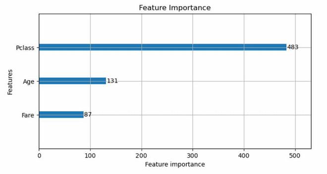
Feature Importance

We are displaying a LightGBM model’s feature relevance with this code. The significance of every feature in the model is displayed in a bar plot created by the lgb.plot_importance() method. Higher significance feature values are thought to have stronger predictive power. We add a title, set the plot’s figsize to control its proportions, then use plt.show() to display the plot.

Advantages

• Efficiency: LightGBM is known for its high efficiency in terms of both training and prediction. It uses a histogram-based algorithm and can handle large datasets with millions of rows and thousands of features quickly.
• Memory Efficiency: It consumes less memory compared to other gradient boosting libraries, making it suitable for environments with limited memory resources.
• Parallel and Distributed Computing: LightGBM supports parallel and distributed computing, allowing for faster training on multi-core CPUs and distributed environments, which can significantly speed up the training process.
• Categorical Feature Handling: LightGBM has built-in support for handling categorical features, and it efficiently encodes them without the need for extensive preprocessing. This is especially valuable when dealing with datasets that contain non-numeric data.
• Accuracy: LightGBM often provides state-of-the-art performance in terms of predictive accuracy. It’s capable of building highly accurate models, making it suitable for a wide range of machine learning tasks.

Disadvantages

• Overfitting: Like other gradient boosting algorithms, LightGBM can be prone to overfitting if not properly tuned. Regularization techniques and careful hyperparameter tuning are often necessary to mitigate this risk.
• Lack of Interpretability: While it provides feature importance scores, LightGBM models are generally considered less interpretable compared to simpler models like linear regression. Understanding how the model arrives at a particular prediction can be challenging.
• Limited in Unstructured Data: LightGBM is most effective with structured data that contains tabular features. It may not be the best choice for tasks involving unstructured data like text or image analysis.
• Less Robustness to Noisy Data: LightGBM can be sensitive to noisy or outlier data. Outliers can have a significant impact on the model’s performance, and preprocessing may be required to handle such situations.
• Black-Box Nature: LightGBM is a gradient boosting algorithm, which is inherently a black-box model. It provides limited insight into how the model makes decisions, which may be problematic in applications where interpretability is crucial.