Handling categorical features with CatBoost

Handling categorical features is an important aspect of building Machine Learning models because many real-world datasets contain non-numeric data which should be handled carefully to achieve good model performance. From this point of view, CatBoost is a powerful gradient-boosting library that is specifically designed for handling categorical features efficiently. In this article, we will discuss how we can handle categorial features by CatBoost.

What is CatBoost

CatBoost or Categorical Boosting is a machine learning algorithm that was developed by Yandex, a Russian multinational IT company. This special boosting algorithm is based on the gradient boosting framework which is specially designed to handle categorical features more effectively than traditional gradient boosting algorithms. CatBoost incorporates techniques like ordered boosting, oblivious trees, and advanced handling of categorical features to achieve high performance with minimal hyperparameter tuning.

What are Categorial Features

Categorical features are variables that represent categories or labels rather than numerical values which are known as nominal or discrete features for this reason. These features are very common in various real-world datasets and can be challenging to work with in machine-learning models. We can divide categorical into two main types:

1. Nominal Categorical Features: These features represent categories with no inherent order or ranking which include “color”, “gender”, “country” etc. These features often require special encoding like Label encoding to be used in machine learning models.
2. Ordinal Categorical Features: These features represent categories with a meaningful order or ranking which include “education level” with categories like “high school”, “bachelor’s degree”, “master’s degree” etc. These features may be encoded with integer values to reflect their order.

Parameters of Catboost

With a multitude of parameters to adjust and refine its models, CatBoost is a robust gradient boosting library. Now let’s look at some of the crucial CatBoost parameters that are frequently used:

• iterations: The total number of ensemble trees or boosting iterations. While more iterations may improve model performance, they also raise the possibility of overfitting. A few hundred to a few thousand are typical values.
• learning_rate: As it approaches the loss function’s minimum, it regulates the step size at each iteration. Although it takes longer iterations, a lower learning rate strengthens the training. The range of common values is 0.01 to 0.3.
• depth: The trees in the ensemble’s depth. It establishes the level of intricacy in each tree. Although they may model complicated relationships, deeper trees run the risk of overfitting. Values typically fall between 4 and 10.
• l2_leaf_reg: The weight-based L2 regularization term. Penalizing heavy weights on features helps avoid overfitting. Better regularization can be achieved by adjusting this parameter.
• random_seed: The random number generator’s seed. Reproducibility of outcomes is ensured by setting this value.
• verbose: It shows the training progress during iterations if set to True. It operates silently and doesn’t print progress if set to False.
• cat_features: An array of indices for categorical features. CatBoost automatically encodes these features for training and handles them differently.
• one_hot_max_size: The maximum number of distinct categories that one-hot encoding of a categorical feature is permitted to have. CatBoost uses an effective technique to handle the feature differently if there are more unique categories than this threshold.

Implementation of Handling categorical features with CatBoost

Installing required modules

At first, we need to install all required Python modules to our runtime.

!pip install catboost
!pip install shap

Importing required libraries

Now we will import all required Python libraries like NumPy, Matplotlib, Seaborn, Pandas and SKlearn etc.

Python3

import pandas as pd
from catboost import CatBoostClassifier, Pool
from sklearn.model_selection import train_test_split
from sklearn.metrics import accuracy_score, classification_report
import matplotlib.pyplot as plt
import seaborn as sns
import shap

Dataset loading and splitting

Python3

# Load the Titanic dataset
url = "https://web.stanford.edu/class/archive/cs/cs109/cs109.1166/stuff/titanic.csv"
df = pd.read_csv(url)

# Select relevant features and target variable
X = df[['Pclass', 'Sex', 'Age', 'Fare']]
y = df['Survived']

# Split the data into training and testing sets
X_train, X_test, y_train, y_test = train_test_split(X, y, test_size=0.3, random_state=42)

Using Pandas, this method loads the Titanic dataset from a given URL. It chooses ‘Survived’ as the target variable (y) and certain attributes (‘Pclass,’Sex,’Age,’Fare’) as input variables (X). Next, using a random state of 42 for repeatability, it divides the data into training and testing sets with a 70% training and 30% testing split.

Exploratory Data Analysis

Examining, condensing, and visualizing a dataset in order to obtain understanding and comprehend its features is known as exploratory data analysis, or EDA. It is an essential phase in the data analysis process. EDA searches the data for correlations, patterns, anomalies, and possible trends.

Correlation matrix

Visualizing correlation matrix between features will help us to understand how the features are related to each other and also helpful for feature selection or engineering.

Python3

# Calculate the correlation matrix
corr_matrix = df.corr(numeric_only=True)

# Create a heatmap to visualize the correlation matrix
plt.figure(figsize=(6, 4))
sns.heatmap(corr_matrix, annot=True, cmap='coolwarm', linewidths=0.5)
plt.title('Correlation Matrix')
plt.show()

Output:

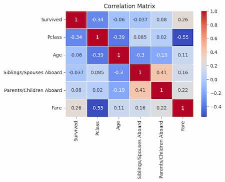
This program uses Pandas’ corr method to compute the correlation matrix for the Titanic dataset’s numeric columns. To see the correlations between these numerical features, it then uses Seaborn to build a heatmap. For improved visibility, a “coolwarm” color map with faint white lines separating the cells is employed, and correlation values are indicated on the heatmap. Plot is presented and has the title “Correlation Matrix” set.

Distribution of target classes

Now we will see how the classes of target feature is distributed. It will help to understand the class distribution which is essential for assessing class balance and potential data biases.

Python3

# Select the target feature
target_feature = 'Survived'

# Create a count plot to visualize the distribution of the target feature
plt.figure(figsize=(4, 3))
sns.countplot(data=df, x=target_feature)
plt.xlabel(target_feature)
plt.ylabel('Count')
plt.title(f'Distribution of {target_feature}')
plt.show()

Output:

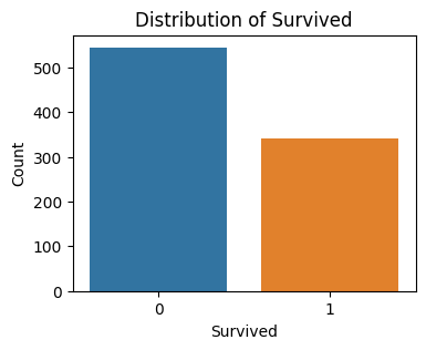
Distribution of target class(Survived) for Titanic Dataset

The Titanic dataset’s target variable, “Survived,” is set to the target_feature variable using this code. It then uses Seaborn to build a count plot so that the distribution of the ‘Survived’ feature can be seen. Whereas the y-axis displays the number of occurrences, the x-axis depicts the ‘Survived’ feature. The plot is displayed and has the title “Distribution of Survived” set.

Distribution of classes for categorial features for Pclass

As we are going to handle categorial features using CatBoost, it is required to know what are the number of categories present and their distribution for a particular categorial feature. In the Titanic dataset there are two categorial features which are ‘Pclass’ and ‘Sex’.

Python3

# Select a single categorical feature
categorical_feature = 'Pclass'

# Create a count plot to visualize the distribution of categories
plt.figure(figsize=(4, 3))
sns.countplot(data=df, x=categorical_feature)
plt.xlabel(categorical_feature)
plt.ylabel('Count')
plt.title(f'Distribution of {categorical_feature}')
plt.show()

Output:

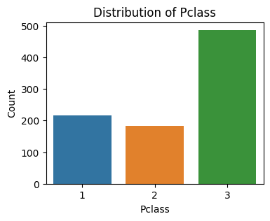
Distribution of categorial feature: Pclass

One categorical feature from the Titanic dataset, ‘Pclass,’ is the value that this code assigns to the categorical_feature variable. It then uses Seaborn to build a count plot so that the distribution of categories inside the ‘Pclass’ feature can be seen. The categories of the ‘Pclass’ characteristic are represented by the x-axis, and the number of occurrences for each category is displayed on the y-axis.

Distribution of classes for categorial features for Sex Column

Python3

# Select a single categorical feature
categorical_feature = 'Sex'

# Create a count plot to visualize the distribution of categories
plt.figure(figsize=(4, 3))
sns.countplot(data=df, x=categorical_feature)
plt.xlabel(categorical_feature)
plt.ylabel('Count')
plt.title(f'Distribution of {categorical_feature}')
plt.show()

Output:

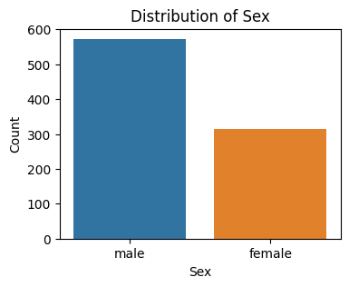
Distribution of categorial feature: Sex

Other categorical feature from the Titanic dataset, “Sex,” is chosen as the value for the categorical feature variable using this code. To show the distribution of categories within the ‘Sex’ feature, it then uses Seaborn to build a count plot. Category counts for the ‘Sex’ feature are displayed on the y-axis, while category counts are represented on the x-axis.

Model Training

Python3

# Create a CatBoost Classifier
cat_features = ['Pclass', 'Sex']  # List of categorical features
one_hot_max_size = 10
model = CatBoostClassifier(iterations=100, depth=6, learning_rate=0.1,
                           verbose=False, cat_features=cat_features, one_hot_max_size=one_hot_max_size)

# Fit the model to the training data
model.fit(X_train, y_train)

Now we will train our CatBoost classifier model by specifying different parameters which are listed below:

By setting up a model with particular hyperparameters, including the number of iterations, tree depth, and learning rate, we may develop a CatBoost Classifier. To tell the model which characteristics are categorical, we provide a list of those features as the cat_features option. Furthermore, we limit one-hot encoding for categorical features with up to 10 unique values by setting one_hot_max_size to 10. To discover the underlying patterns and relationships in the data, we fit (train) the model using the training set (X_train and y_train). During the fitting procedure, detailed training output is suppressed by setting the verbose parameter to False.

one_hot_max_size: The most distinct categories that can be used for one-hot encoding in a categorical feature. CatBoost uses the one_hot_max_size parameter to regulate how one-hot encoding for categorical features behaves. It indicates the most distinct categories that can exist in a categorical feature before it is one-hot encoded. CatBoost will encrypt a feature in one-hot fashion if its unique category count is less than or equal to one_hot_max_size.

Model Evaluation

Now we will evaluate our model’s performance in the terms of accuracy and classification report.

Accuracy

Python3

# Make predictions
y_pred = model.predict(X_test)
# Evaluate the model
accuracy = accuracy_score(y_test, y_pred)
print(f"Accuracy: {accuracy:.2f}")

Output:

Accuracy: 0.82

This code uses the learned CatBoost model to make predictions (y_pred) on the test data (X_test). By comparing the model’s predictions to the actual target values (y_test), we can determine the accuracy of the predictions. The accuracy score is then displayed.

Classification Report

Python3

#classification Report
classification_rep = classification_report(y_test, y_pred)
print("Classification Report:\n", classification_rep)

Output:

Classification Report:
               precision    recall  f1-score   support
           0       0.80      0.95      0.87       166
           1       0.87      0.60      0.71       101
    accuracy                           0.82       267
   macro avg       0.83      0.77      0.79       267
weighted avg       0.83      0.82      0.81       267

Using the scikit-learn classification_report function, we produce a classification report (classification_rep). Based on the predicted and true target values, it computes a number of classification metrics for each class, including support, recall, F1-score, and accuracy. To give a thorough overview of the model’s success in classifying the test data, we print the classification report.

Visualization of features Shap values

Shap values visualization of all categorial and non-categorial features will help us to understand which features contributed how much to make the model prepared for prediction.

Python3

# Explain feature importance using SHAP
explainer = shap.Explainer(model)
shap_values = explainer.shap_values(X_test)

# Create a summary plot
shap.summary_plot(shap_values, X_test, plot_type="bar", plot_size= 0.2)
plt.show()

Output:

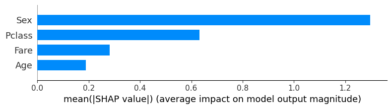
Shap values of features plot

The feature importance of the CatBoost model is explained in this code using SHAP (SHapley Additive exPlanations). With the test data, it generates an explanation object to calculate SHAP values for the model’s predictions. Each feature’s contribution to the model’s output is shown by the SHAP values. In order to illustrate the feature relevance based on the SHAP values, the shap.summary_plot method creates a summary plot in bar style. The most important characteristics for the model’s predictions are revealed through the plot.

Conclusion

We can conclude that, we should always be cautious when handling categorial features of any dataset because these features are very crucial to make a optimized model which accurate predictions. Our model has achived good accuracy of 82%. However, using more complex dataset where more number of categorial features are there can degrade this accuracy. In that case, we should perform hyper-parameter tuning of CatBoost model.