Fuzzy Clustering in R

Clustering is an unsupervised machine-learning technique that is used to identify similarities and patterns within data points by grouping similar points based on their features. These points can belong to different clusters simultaneously. This method is widely used in various fields such as Customer Segmentation, Recommendation Systems, Document Clustering, etc. It is a powerful tool that helps data scientists identify the underlying trends in complex data structures. In this article, we will understand the use of fuzzy clustering with the help of multiple real-world examples.

Understanding Fuzzy Clustering

In real-world scenarios, these clusters can belong to multiple other different clusters. Fuzzy clustering addresses this limitation by allowing data points to belong to multiple clusters simultaneously. In R Programming Language is widely used in research, academia, and industry for various data analysis tasks. It has the following advantages over normal clustering:

• Soft Boundaries: Fuzzy clustering provides soft boundaries allowing data points to belong to multiple other clusters simultaneously. This is a realistic approach to data handling.
• Robustness to Noisy Data: It can handle noise better than traditional clustering algorithms.
• Flexibility: As mentioned earlier there is flexibility for data points to belong to multiple clusters. This helps in the study of complex data structures.

Difference between Normal and Fuzzy Clustering

Factor	Normal Clustering	Fuzzy Clustering
Partitioning	Hard Partitioning, data points can belong to only one cluster.	Soft Partitioning, data points can belong to multiple clusters.
Membership	Data points can either belong to one cluster or none at all.	Data points can belong to multiple clusters simultaneously.
Representation	represented by centroids.	represented by centroids with degrees of membership
Suitable dataset	Dataset with distinct boundaries	Dataset with overlapping observations
Algorithm used	K-means, Hierarchical clustering	Fuzzy C -means, Gustafson-Kessel algorithm
Implementation	Easier to implement since the dataset is not complex	Difficult to Implement since dataset has overlapping observations

Implementation of Fuzzy Clustering

To apply fuzzy clustering to our dataset we need to follow certain steps.

1. Loading Required Libraries
2. Loading the Dataset
3. Data Preprocessing
4. Data Selection for Clustering
5. Fuzzy C-means Clustering
6. Interpret the Clustering Results
7. Visualizing the Clustering Results

Important Packages

• e1071: This package is widely used in statistical analysis because of its tools for implementation of machine learning algorithms. It is used for regression tasks, clustering, and data analysis. The main purpose of this package is to provide support to various machine learning algorithms such as support vector machines (SVM), naive Bayes, and decision trees making it a popular choice for data scientists.
• cluster: This package in R is used for clustering whether it is K-means clustering, hierarchical clustering, or fuzzy clustering. It helps in analyzing and visualizing clusters within a dataset.
• factoextra: This package is used for multivariate data extraction and visualization of complex datasets.
• ggplot2: ggplot2 library stands for grammar of graphics, popular because of its declarative syntax used to visualize and plot our data into graphs for better understanding.
• plotly: This is another package used for data visualization which allows users to create interactive graphs. It supports various programming langauges such as R, Julia, Python, etc. It allows various features to create basic charts, statistical graphs, 3-D plots, etc.
• fclust: This package in R provides a set of tools for fuzzy clustering analysis. It includes various algorithms for fuzzy clustering and analyzing the results. There are certain key features and functions of this package:
• fanny(): This function is used for implementing the Fuzzy- C Means algorithm by providing multiple parameters for our datasets.
• cplot(): The versatility of this package allows us to plot the clusters, this function helps us in plotting them.
• validityindex(): This function helps in understanding the quality of the results. This is used for performance analysis.
• readxl : This package helps in importing excel files in R environment for further analysis.
• fpc: This package provides various functions for fundamental clustering tasks and cluster evaluation metrics
• clusterSim: This package is an R package that provides a set of tools for assessing and comparing clustering results.
• scatterplot3d: As the name suggests, this library is used to plot the 3-dimensional graphs for visualization.
  We can understand this topic in a better way by dealing with various diverse problems based on real-world issues.

Fuzzy Clustering in R using Customer Segmentation datset

In this example we will apply fuzzy clustering on a Sample sales dataset which we will download from the Kaggle website. You can download it from https://www.kaggle.com/datasets/kyanyoga/sample-sales-data
This dataset contains data about Order Info, Sales, Customer, Shipping, etc., which is used for analysis and clustering. We will follow the code implementation steps that is needed.

1. Loading Required Libraries

As discussed above the libraries that we need for clustering are e1071, cluster, factoextra, ggplot2 and their roles are already mentioned. Syntax to install and load these libraries are:

R

# Install libraries
install.packages("e1071")
install.packages("cluster")
install.packages("factoextra")
#load libraries
library(e1071)
library(cluster)
library(factoextra)

2.Loading the Dataset

This part of the code reads the dataset by the provided path. You can replace the name from the path of your actual file.

R

data <- read.csv("your_path.csv")

head(data)

Output:

 ORDERNUMBER QUANTITYORDERED PRICEEACH ORDERLINENUMBER   SALES       ORDERDATE
1       10107              30     95.70               2 2871.00  2/24/2003 0:00
2       10121              34     81.35               5 2765.90   5/7/2003 0:00
3       10134              41     94.74               2 3884.34   7/1/2003 0:00
4       10145              45     83.26               6 3746.70  8/25/2003 0:00
5       10159              49    100.00              14 5205.27 10/10/2003 0:00
6       10168              36     96.66               1 3479.76 10/28/2003 0:00
   STATUS QTR_ID MONTH_ID YEAR_ID PRODUCTLINE MSRP PRODUCTCODE
1 Shipped      1        2    2003 Motorcycles   95    S10_1678
2 Shipped      2        5    2003 Motorcycles   95    S10_1678
3 Shipped      3        7    2003 Motorcycles   95    S10_1678
4 Shipped      3        8    2003 Motorcycles   95    S10_1678
5 Shipped      4       10    2003 Motorcycles   95    S10_1678
6 Shipped      4       10    2003 Motorcycles   95    S10_1678
              CUSTOMERNAME            PHONE                  ADDRESSLINE1
1        Land of Toys Inc.       2125557818       897 Long Airport Avenue
2       Reims Collectables       26.47.1555            59 rue de l'Abbaye
3          Lyon Souveniers +33 1 46 62 7555 27 rue du Colonel Pierre Avia
4        Toys4GrownUps.com       6265557265            78934 Hillside Dr.
5 Corporate Gift Ideas Co.       6505551386               7734 Strong St.
6     Technics Stores Inc.       6505556809             9408 Furth Circle
  ADDRESSLINE2          CITY STATE POSTALCODE COUNTRY TERRITORY CONTACTLASTNAME
1                        NYC    NY      10022     USA      <NA>              Yu
2                      Reims            51100  France      EMEA         Henriot
3                      Paris            75508  France      EMEA        Da Cunha
4                   Pasadena    CA      90003     USA      <NA>           Young
5              San Francisco    CA                USA      <NA>           Brown
6                 Burlingame    CA      94217     USA      <NA>          Hirano
  CONTACTFIRSTNAME DEALSIZE
1             Kwai    Small
2             Paul    Small
3           Daniel   Medium
4            Julie   Medium
5            Julie   Medium
6             Juri   Medium

3. Data Preprocessing

na.omit() function helps in removing rows that have missing values. These missing values can alter our analysis so dealing with them is important.

R

# column wise missing values
colSums(is.na(data))

# Handle missing values
data<- na.omit(data)

Output:

     ORDERNUMBER  QUANTITYORDERED        PRICEEACH  ORDERLINENUMBER            SALES 
               0                0                0                0                0 
       ORDERDATE           STATUS           QTR_ID         MONTH_ID          YEAR_ID 
               0                0                0                0                0 
     PRODUCTLINE             MSRP      PRODUCTCODE     CUSTOMERNAME            PHONE 
               0                0                0                0                0 
    ADDRESSLINE1     ADDRESSLINE2             CITY            STATE       POSTALCODE 
               0                0                0                0                0 
         COUNTRY        TERRITORY  CONTACTLASTNAME CONTACTFIRSTNAME         DEALSIZE 
               0             1074                0                0                0 

4. Data Selection for Clustering

Our dataset is huge, therefore we need to select the columns we wanna deal with. Here, we will perform clustering on Quantity ordered, price each, sales and manufacturer’s suggested retail price. You can get the column names by colnames() syntax in R.

R

data_for_clustering <- data[, c("QUANTITYORDERED", "PRICEEACH", "SALES", "MSRP")]

5. Fuzzy C-means Clustering

Now, we will perform clustering on our selected data for which we use cmeans() function. It defines the number of clusters as well as fuzziness coefficient.

R

set.seed(123)
n_cluster <- 5
m <- 2
result <- cmeans(data_for_clustering, centers = n_cluster, m = m)

Data Membership Degree Matrix:

The Data Membership Degree Matrix, also known as the Fuzzy Membership Matrix, is a fundamental concept in fuzzy clustering algorithms which shows the degree to which each data point belongs to each of the clusters. These values typically range between 0 and 1, where 0 indicates no membership, and 1 indicates full membership.

R

# Data Membership Degree Matrix
fuzzy_membership_matrix <- result$membership

# Cluster Prototype Evolution Matrices
initial_centers <- result$centers
final_centers <- t(result$centers)

6. Interpret the Clustering Results

R

cluster_membership <- as.data.frame(result$membership)
data_with_clusters <- cbind(data, cluster_membership)
head(data_with_clusters)

Output:

   ORDERNUMBER QUANTITYORDERED PRICEEACH ORDERLINENUMBER   SALES       ORDERDATE
2        10121              34     81.35               5 2765.90   5/7/2003 0:00
3        10134              41     94.74               2 3884.34   7/1/2003 0:00
7        10180              29     86.13               9 2497.77 11/11/2003 0:00
8        10188              48    100.00               1 5512.32 11/18/2003 0:00
10       10211              41    100.00              14 4708.44  1/15/2004 0:00
11       10223              37    100.00               1 3965.66  2/20/2004 0:00
    STATUS QTR_ID MONTH_ID YEAR_ID PRODUCTLINE MSRP PRODUCTCODE
2  Shipped      2        5    2003 Motorcycles   95    S10_1678
3  Shipped      3        7    2003 Motorcycles   95    S10_1678
7  Shipped      4       11    2003 Motorcycles   95    S10_1678
8  Shipped      4       11    2003 Motorcycles   95    S10_1678
10 Shipped      1        1    2004 Motorcycles   95    S10_1678
11 Shipped      1        2    2004 Motorcycles   95    S10_1678
                 CUSTOMERNAME            PHONE                  ADDRESSLINE1
2          Reims Collectables       26.47.1555            59 rue de l'Abbaye
3             Lyon Souveniers +33 1 46 62 7555 27 rue du Colonel Pierre Avia
7    Daedalus Designs Imports       20.16.1555       184, chausse de Tournai
8                Herkku Gifts    +47 2267 3215   Drammen 121, PR 744 Sentrum
10           Auto Canal Petit   (1) 47.55.6555             25, rue Lauriston
11 Australian Collectors, Co.     03 9520 4555             636 St Kilda Road
   ADDRESSLINE2      CITY    STATE POSTALCODE   COUNTRY TERRITORY CONTACTLASTNAME
2                   Reims               51100    France      EMEA         Henriot
3                   Paris               75508    France      EMEA        Da Cunha
7                   Lille               59000    France      EMEA           Rance
8                  Bergen              N 5804    Norway      EMEA          Oeztan
10                  Paris               75016    France      EMEA         Perrier
11      Level 3 Melbourne Victoria       3004 Australia      APAC        Ferguson
   CONTACTFIRSTNAME DEALSIZE            1           2            3            4
2              Paul    Small 0.0001541063 0.999690200 0.0001263451 2.272976e-05
3            Daniel   Medium 0.0048451207 0.020573748 0.9663439156 6.979966e-03
7           Martine    Small 0.0878851450 0.874531088 0.0290942132 6.458913e-03
8            Veysel   Medium 0.0045450830 0.009277472 0.0321427220 9.454499e-01
10        Dominique   Medium 0.0290347397 0.075020298 0.6323656865 2.425679e-01
11            Peter   Medium 0.0011707987 0.004626692 0.9918892502 1.975149e-03
              5
2  6.618887e-06
3  1.257249e-03
7  2.030640e-03
8  8.584810e-03
10 2.101140e-02
11 3.381099e-04

head() function prints the first few rows of our dataset. The results we got can be divided into four parts for better understanding:

• Customer Details: This sections gives information about the individual customer such as order number, quantity ordered, price each, total sales, order date, product information, name, etc, to identify each customer individually.
• Cluster Membership Probabilities: Column 1 to 5 shows the probabilities of a customer belonging to a certain cluster generated by our algorithm.
• Deal Size Classification: This category can hold three values, small, medium and large in our dataset but the results that we got has just small and medium based on the size of the deal.
• Understanding Customer Behavior: This is the main purpose of our analysis since we are dividing our customers into different clusters to understand their purchasing behaviour. This clustering will help us understand the buying patterns and give better recommendation to that cluster or group of customers. Clustering in such cases also helps in improving customer services.

Cluster Separation Score or Gap Index

Cluster Separation Score or Gap Index is used calculate the optimal number of clusters in our dataset. Higher gap index suggests better defined clusters.
It measures the gap between the observed clustering quality and the expected clustering quality

R

# Load required libraries
library(clusterSim)

# Clustering Comparison for Determining Optimal Clusters

# Computing PAM clustering with k = 4
cl1 <- pam(data_for_clustering, 4)

# Computing PAM clustering with k = 5
cl2 <- pam(data_for_clustering, 5)

# Combine the clustering results
cl_all <- cbind(cl1$clustering, cl2$clustering)

# Calculate the Gap index for the dataset
gap <- index.Gap(data_for_clustering, cl_all, reference.distribution = "unif",
                 B = 10, method = "pam")

# Print the Gap index
print(gap)

Output:

$gap
[1] 0.3893237
$diffu
[1] -0.1060642

gap index(gap) : represents distinct and quality clusters. The value we got here shows a moderate level of distinctiveness and separation between clusters.
difference values(diffu) : represents the uncertainty in the estimated Gap statistic. A negative value here indicates that the clustering solution has a lower standard deviation which shows that the clusters are distinct in comparison to random distribution.
Together these values help in estimating the quality of clusters.

Davies-Bouldin’s index

This Index is useful in finding the similarities between the clusters. This deals with both the scatter within the clusters and the separation between the clusters for model fit. A lower Davies-Bouldin’s index indicates better clustering.

R

# Load required libraries
library(cluster)

# Calculate PAM clustering with k = 5
clustering_results <- pam(data_for_clustering, 5)
# Calculate Davies-Bouldin's index for the dataset
db_index <- index.DB(data_for_clustering, clustering_results$clustering,
                     centrotypes = "centroids")

# Print Davies-Bouldin's index
print(db_index)

Output:

$DB
[1] 0.6708421
$r
[1] 0.6288000 0.5934592 0.7515756 0.7515756 0.6288000
$R
          [,1]      [,2]      [,3]      [,4]      [,5]
[1,]       Inf 0.5934592 0.2948785 0.3190663 0.6288000
[2,] 0.5934592       Inf 0.5603336 0.4305076 0.3335226
[3,] 0.2948785 0.5603336       Inf 0.7515756 0.2264422
[4,] 0.3190663 0.4305076 0.7515756       Inf 0.2724843
[5,] 0.6288000 0.3335226 0.2264422 0.2724843       Inf
$d
         1        2        3        4        5
1    0.000 1142.226 2635.563 4947.227 1088.237
2 1142.226    0.000 1493.378 3805.072 2230.441
3 2635.563 1493.378    0.000 2311.701 3723.724
4 4947.227 3805.072 2311.701    0.000 6035.324
5 1088.237 2230.441 3723.724 6035.324    0.000
$S
[1]  309.1230  368.7419  468.0478 1269.3704  375.1605
$centers
         [,1]     [,2]     [,3]      [,4]
[1,] 33.48421 81.46667 2704.752  89.80421
[2,] 35.98091 94.16315 3846.702 111.30788
[3,] 41.05263 99.80880 5339.980 126.80827
[4,] 45.48344 99.95550 7651.551 150.98013
[5,] 28.18721 59.94959 1616.948  68.52968

• $DB: The value of Davies-Bouldin’s index for the clustering result.
• $r: These value represent the average distances between each point in one cluster to every other point in the same cluster.
• $R: These value represent between the centroids of different clusters.
• $d: These value represent the distance between each pair of data points.
• $S: The scatter values for each cluster.
• $centers: The coordinates of the cluster centers for each variable

Variance Ratio Criterion or Calinski-Harabasz index

This parameter is used to calculate the ratio between the variance between the clusters and variance within the clusters. A higher value is preferred as it suggests better defined clusters and clear separation between them.
PAM is a partitional clustering method used to create clusters with actual data points.

R

# Cluster Evaluation using Calinski-Harabasz Index

# Calculate PAM clustering with k = 10
clustering_results <- pam(data_for_clustering, 10)
# Calculate Calinski-Harabasz pseudo F-statistic for the dataset
ch_index <- index.G1(data_for_clustering, clustering_results$clustering)

# Print the Calinski-Harabasz pseudo F-statistic
print(ch_index)

Output:

[1] 7433.806

This code first performance PAM clustering on 10 clusters and then computers Variance Ratio Criterion for the results we got by clustering. The output we got suggests that the data points are well separated into distinct clusters, with minimal variations within each cluster. This output suggest better clustering performance.

7. Visualizing the Clustering Results

Now to visualize the results we will use “ggplot2” the famous package used for plotting graphs.

R

centers <- t(result$centers)
data_with_clusters$Cluster <- apply(result$membership, 1, which.max)
ggplot(data_with_clusters, aes(x = QUANTITYORDERED, y = PRICEEACH,
                               color = as.factor(Cluster))) +
  geom_point() +
  labs(title = "Fuzzy C-means Clustering", x = "Quantity Ordered", y = "Price Each")

Output:

Fuzzy Clustering in R

Each color represents the different clusters of the customers that have same purchasing habits. The data points represents the relationship for the customer about the quantity of their order and the price for their order. This gives insights on the customer segmentation.

Variable Relationships Visualization:

Variable Relationship Plots are made to understand the relationship between the variables present in our dataset. Pairwise scatter plots visualize the relationships between pairs of variables, aiding in identifying patterns and relationships between features. This graph also helps in identifying the potential relationship

R

pairs(data_for_clustering, pch = 16, col = as.numeric(result$cluster))

Output:

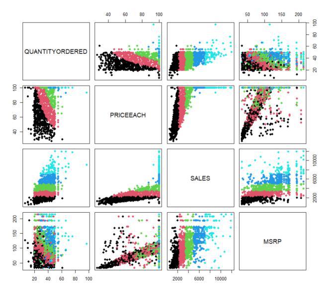
Variable Relationships Visualization

Scatter plots illustrate how ‘QUANTITYORDERED’ and ‘PRICEEACH’ or ‘SALES’ and ‘MSRP’ are related, highlighting any trends or correlations in the data. This helps in identifying both underlying trends as well as potential relations.

Data Point Cluster Representation or Clusplot refers to visualization of data points in relation to their clusters. This is another visualization technique to analyze clusters, which provides a different perspective on the distribution and relationships between clusters. This plot helps to understand how each data point is distributed and belongs to a certain cluster based on their features or attributes.

Data Point Cluster Representation Another visualization technique to analyze clusters, which provides a different perspective on the distribution and relationships between clusters.

R

clusplot(data_for_clustering, result$cluster, color = TRUE, shade = TRUE,
clusplot(data_for_clustering, result$cluster, color = TRUE, shade = TRUE,
         labels = 2, lines = 0))

Output:

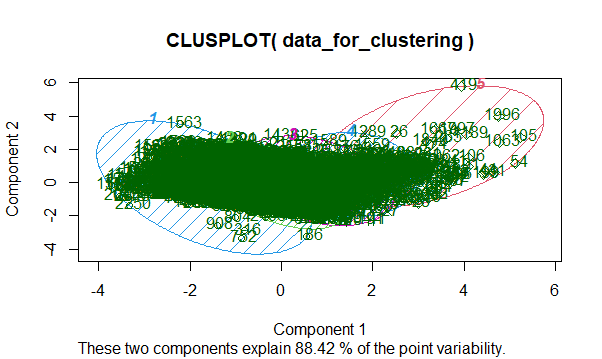
Fuzzy Clustering in R

A higher percentage of point variability between the variables represents that the clusters can be distributed into distinct clusters based on the components. The graph appears to be complex since we have too many datasets. Here 88.42% of the point variability shows that if we are working a large dataset then these two components are useful on determining the main characteristics of the dataset we have. These two components will help us to understand and see main patterns.

This analysis is important to understand the purchasing patterns of the customers for a particular business. These segmentations help in making informed decisions such as making strategies or recommendations which helps in improving customer satisfaction. It also helps in improving customer engagement by providing personalized recommendations.

Fuzzy Clustering in R on Medical Diagnosis dataset

1. Loading Required Libraries

R

# Loading Required Libraries
# For fuzzy clustering
library(e1071)
library(ggplot2)

2. Loading the Dataset

We are creating a fictional dataset about patient health parameters. Synthetic data is created for 100 patients, the parameters that are used here are : blood pressure, cholesterol and BMI(body mass index).

R

# Loading the Dataset
set.seed(123)  # for reproducibility
patients <- data.frame(
  patient_id = 1:100,
  blood_pressure = rnorm(100, mean = 120, sd = 10),
  cholesterol = rnorm(100, mean = 200, sd = 30),
  bmi = rnorm(100, mean = 25, sd = 5)
)

3. Data Preprocessing

This step is important to ensure that all the variables are on the same scale, this is a common practice done in clustering.

R

# Data Preprocessing
scaled_data <- scale(patients[, -1])

4. Data Selection for Clustering

This segment involve selecting relevant variables for clustering.

R

# Data Selection for Clustering
selected_data <- scaled_data[, c("blood_pressure", "cholesterol", "bmi")]

5. Fuzzy C-means Clustering with FGK Algorithm

The Fuzzy Gustafson-Kessel (FGK) algorithm is a variant of the Fuzzy C-means (FCM) clustering algorithm which focuses on overlapping clusters. It works with dataset that are overlapping and have non-spherical clustering. he membership grades are determined based on the weighted Euclidean distance between data points and cluster centers. Euclidean Distance formula is used to measure straight line distance between two points in Euclidean space. The formula is given by:

d = √[ (x2– x1) 2  + (y2– y1 )2]

• where (x₁, y₁) are the coordinates of one point
• and (y₁, y₂) are the coordinates of other point.
• and d is the distance between them

R

# Fuzzy C-means Clustering with FGK algorithm
set.seed(456)
fgk_clusters <- e1071::cmeans(selected_data, centers = 3, m = 2)$cluster

selected_data refers to the selected columns we need for clustering. Number of centers here are 3 and High value of m shows fuzzier cluster.

Data Membership Degree Matrix and the Cluster Prototype Evolution Matrices

In fuzzy clustering each data point is assigned with a degree of membership which defines the degree of belongingness of that data point to a definite cluster whereas the cluster prototype evolution matrices are used to show the change in centroid position over the iteration.

R

# Fuzzy C-means Clustering with FGK algorithm
set.seed(456)  # for reproducibility
fuzzy_result <- e1071::cmeans(selected_data, centers = 3, m = 2)

# Access the membership matrix and cluster centers
membership_matrix <- fuzzy_result$membership
cluster_centers <- fuzzy_result$centers

# Print the membership matrix and cluster centers
print("Data Membership Degree Matrix:")
print(membership_matrix)

print("Cluster Prototype Evolution Matrices:")
print(cluster_centers)

Output:

"Data Membership Degree Matrix:"
        1          2          3
  [1,] 0.15137740 0.15999978 0.68862282
  [2,] 0.10702292 0.19489294 0.69808414
  [3,] 0.71018858 0.18352624 0.10628518
  [4,] 0.21623783 0.18849017 0.59527200
  [5,] 0.70780116 0.14281776 0.14938109
  [6,] 0.63998321 0.23731396 0.12270283
  [7,] 0.82691960 0.10470764 0.06837277
  [8,] 0.33246815 0.25745565 0.41007620
  [9,] 0.08219287 0.10368827 0.81411886
 [10,] 0.06659943 0.83694230 0.09645826....
[100,] 0.12656903 0.12155473 0.75187624

"Cluster Prototype Evolution Matrices:"
 blood_pressure cholesterol        bmi
1      0.6919000  -0.5087515 -0.4642972
2     -0.1031542   0.7724248 -0.3050143
3     -0.6279179  -0.3104457  0.8176061

The higher values show a strong relationship between the clusters and data points as given in our output. All the 100 rows are not represented here, you can get those values by following the code.
The values in the matrix show the movement of the cluster centroids in each dimension of each variable that is blood pressure, cholesterol and bmi.

6. Interpret the Clustering Results

In this step we are combining the clustering results with our original data with the help of cbind() function. summary() function gives us an insight of our data.

R

# Interpret the Clustering Results
clustered_data <- cbind(patients, cluster = fgk_clusters)
summary(clustered_data)

Output:

   patient_id     blood_pressure    cholesterol         bmi           cluster    
 Min.   :  1.00   Min.   : 96.91   Min.   :138.4   Min.   :16.22   Min.   :1.00  
 1st Qu.: 25.75   1st Qu.:115.06   1st Qu.:176.0   1st Qu.:22.34   1st Qu.:1.00  
 Median : 50.50   Median :120.62   Median :193.2   Median :25.18   Median :2.00  
 Mean   : 50.50   Mean   :120.90   Mean   :196.8   Mean   :25.60   Mean   :2.02  
 3rd Qu.: 75.25   3rd Qu.:126.92   3rd Qu.:214.0   3rd Qu.:28.82   3rd Qu.:3.00  
 Max.   :100.00   Max.   :141.87   Max.   :297.2   Max.   :36.47   Max.   :3.00

The summary() shows the min, first quartile, median, 3rd quartile and max of different columns of our dataset. This information can be helpful for the researchers in studying the underlying patterns in the dataset for further decision making.

GAP INDEX

Gap index or Gap statistics is used to calculate the optimal number of clusters withing a dataset. It defines the optimal number of clusters after which adding the cluster number will not play any significant role in analysis.

R

# Function to calculate the gap statistic
gap_statistic <- function(data, max_k, B = 50, seed = NULL) {
  require(cluster)

  set.seed(seed)

  # Compute the observed within-cluster dispersion for different values of k
  wss <- numeric(max_k)
  for (i in 1:max_k) {
    wss[i] <- sum(kmeans(data, centers = i)$withinss)
  }

  # Generate B reference datasets and calculate the within-cluster dispersion for each
  B_wss <- matrix(NA, B, max_k)
  for (b in 1:B) {
    ref_data <- matrix(rnorm(nrow(data) * ncol(data)), nrow = nrow(data))
    for (i in 1:max_k) {
      B_wss[b, i] <- sum(kmeans(ref_data, centers = i)$withinss)
    }
  }

  # Calculate the gap statistic
  gap <- log(wss) - apply(B_wss, 2, mean)
  return(gap)
}

# Example usage of the gap_statistic function
gap_values <- gap_statistic(selected_data, max_k = 10, B = 50, seed = 123)
print(gap_values)

Output:

[1] -286.82712 -209.32084 -163.01342 -131.98106 -112.70612  -98.07825  -87.90545
 [8]  -77.92460  -69.81373  -63.42550

This output suggests that the smaller clusters will be better to present this dataset. The negative values suggest that the observed within-cluster variation is less than the expected variation in the dataset.

Davies-Bouldin’s index

It assess the average similarity between the clusters, it deals with both the scatter within the clusters and the separation between the clusters covering a wide range and helping us in estimating the quality of the clusters.

R

# Function to calculate the Davies-Bouldin index
davies_bouldin_index <- function(data, cluster_centers, membership_matrix) {
  require(cluster)

  num_clusters <- nrow(cluster_centers)
  scatter <- numeric(num_clusters)
  for (i in 1:num_clusters) {
    scatter[i] <- mean(sqrt(rowSums((data - cluster_centers[i,])^2)) * membership_matrix[i,])
  }

  # Calculate the cluster separation
  separation <- matrix(0, nrow = num_clusters, ncol = num_clusters)
  for (i in 1:num_clusters) {
    for (j in 1:num_clusters) {
      if (i != j) {
        separation[i, j] <- sqrt(sum((cluster_centers[i,] - cluster_centers[j,])^2))
      }
    }
  }

  # Calculate the Davies-Bouldin index
  db_index <- 0
  for (i in 1:num_clusters) {
    max_val <- -Inf
    for (j in 1:num_clusters) {
      if (i != j) {
        val <- (scatter[i] + scatter[j]) / separation[i, j]
        if (val > max_val) {
          max_val <- val
        }
      }
    }
    db_index <- db_index + max_val
  }
  db_index <- db_index / num_clusters
  return(db_index)
}

# Example usage of the Davies-Bouldin index function
db_index <- davies_bouldin_index(selected_data, cluster_centers, membership_matrix)
print(paste("Davies-Bouldin Index:", db_index))

Output:

"Davies-Bouldin Index: 0.77109024677212"

Based on our output result which is a lower value it shows that our clusters are well defined and these are well separated from each other.

7. Visualizing the Clustering Results

R

# Visualizing the Clustering Results
ggplot(clustered_data, aes(x = blood_pressure, y = cholesterol,
                           color = factor(cluster))) +
  geom_point(size = 3) +
  labs(title = "Clustering of Patients Based on Health Parameters",
       x = "Blood Pressure", y = "Cholesterol") +
  scale_color_manual(values = c("darkgreen", "green3", "lightgreen")) +
  theme_minimal()

Output:

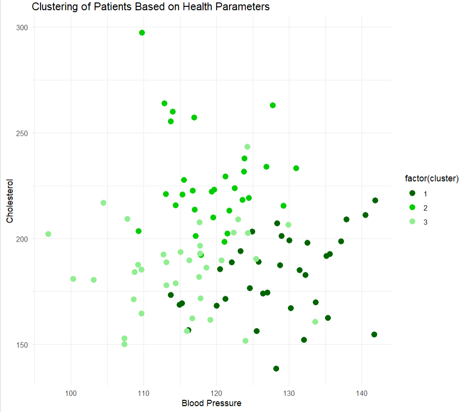
Cholesterol vs Blood pressure graph

In this graph each data point represents a patient defined by the cluster color. The different shades of cluster defines the difference between them.

Data Point Cluster Representation

This information is required since we simplify the complex structure into easier forms for better understanding. This representation can help understand the underlying trends, patterns and complex information that cannot be understood with high dimensional original dataset. It also helps in understanding the outliers that are not easily detectable in the original dataset.

R

# Load the required library
library(cluster)

# Create a data frame including the cluster assignment
clustered_data$cluster <- as.factor(clustered_data$cluster)

# Plot the clusters using clusplot
clusplot(selected_data, clustered_data$cluster, color = TRUE, shade = TRUE,
         labels = 2, lines = 0)

Output:

Data Point Cluster Representation

Different clusters are represented in different colors here and the clusters are also shaded to provide a clear view with each data points. 71.02% of the point variability explains the percentage of variance in the data. This means the two principal components of this data capture 71.02% of variance present in the original dataset.

Variable Relationships Visualization

To visualize the relationship between the variables we plot the pair scatter plot of our dataset. Here we are using pairs() function to create a scatter plot matrix.

R

# Load necessary libraries
library(ggplot2)

# Create a scatter plot matrix
pairs(selected_data, main = "Scatter Plot Matrix of Health Parameters")

Output:

Variable Relationships Visualization

The diagonal elements show the distribution of each variable. This scatter plot helps us to visualize the relationships between different variables, such as blood pressure, cholesterol, and BMI, in the dataset. In the context of patient health parameters, the scatter plot can help us understand how these variables are connected to each other. Understanding these patterns can help us asses the potential risk and help in decision making.

In this example, we created a fictional data set for medical diagnosis using Fuzzy Gustafson-Kessel (FGK) algorithm. We used different packages for clustering the results with the original dataset. Such kind of clustering helps the medical practitioner draw conclusions based on the medical history and similarities between multiple patients and their symptoms. This also makes treatment decisions easier.

Conclusion

In this article, we got to know about different algorithms and their base used for fuzzy clustering and how it helps in various fields such as medical, agriculture, traffic pattern analysis and customer segmentation. We applied this on various type of dataset from different sources. We also plotted the results of these clustering on graph for better visualization. These clustering data points help researchers identify how each of them belong or contribute to different factors and how they affect the study as a whole.