Spectral Clustering: A Comprehensive Guide for Beginners

Clustering plays a crucial role in unsupervised machine learning by grouping data points into clusters based on their similarities. This technique helps us uncover hidden structures and patterns within the data. Spectral clustering, an approach that utilizes properties of graphs and linear algebra, is commonly employed for this purpose. Unlike algorithms like K-Means, spectral clustering is particularly effective in dealing with complex and non-convex data structures. It allows us to explore relationships among data points and has proven valuable in fields such as image segmentation, social network analysis, and community detection.

What is Spectral Clustering?

Spectral Clustering is a technique, in machine learning that groups or clusters data points together into categories. It’s a method that utilizes the characteristics of a data affinity matrix to identify patterns within the data. Spectral clustering has gained popularity across fields, including image segmentation, social network analysis, and community detection.

1. Graph-Based Approach: Spectral Clustering is rooted in graph theory. It treats data points as nodes within a graph, where the connections between nodes represent their pairwise similarity or affinity. This information about affinity is then used to construct a graph.
2. Laplacian Matrix: The central idea behind Spectral Clustering lies in the matrix, which summarizes the relationships, between data points within the graph. There are two types of matrices; unnormalized Laplacian and normalized Laplacian. These matrices capture characteristic aspects of the underlying graph.
3. Eigenvalue Decomposition: The technique known as Spectral Clustering utilizes eigenvalue decomposition on the Laplacian matrix to facilitate cluster identification. Through the computation of eigenvalues and eigenvectors, Spectral Clustering effectively transforms data into a novel space that allows for enhanced separation between clusters. Notably, the eigenvectors associated with smaller eigenvalues often contain valuable insights regarding the underlying structure of clusters.
4. Dimensionality Reduction: In addition to their role in clustering analysis, these eigenvectors can be interpreted as coordinates within a higher-dimensional space. Consequently, one can leverage this property to reduce dimensionality by selecting a subset of these eigenvectors.
5. Cluster Assignment: Following dimensionality reduction, conventional clustering algorithms such as K-Means or hierarchical clustering may then be employed on the reduced data within this new space. This subsequent step facilitates the formation of well-defined clusters based on similarity patterns among data points.

How does Spectral Clustering work?

• Make a graph to show the information. Euclidean distance, cosine similarity, and mutual information are a few examples of similarity metrics that can be used for this.
• Determine the graph’s Laplacian matrix. The graph’s connectedness is represented by the square Laplacian matrix. This is how it is defined:

L = D – W

where W is the graph’s adjacency matrix, a square matrix that contains the similarity between each pair of nodes, and D is the graph’s degree matrix, a diagonal matrix that contains the number of edges associated to each node.

• Find the Laplacian matrix’s eigenvalues and eigenvectors. The inherent structure of the data is captured by the Laplacian matrix’s eigenvalues and eigenvectors.
• Project the data points onto the Laplacian matrix’s leading eigenvectors. The data is converted into a lower-dimensional space where the clusters are more distinctly divided by this dimensionality reduction stage.

Key Concept of Spectral Clustering

Spectral clustering is fundamentally grounded in spectral graph theory, which serves as the underpinning for comprehending its operational mechanism. Spectral graph theory treats data points as nodes within a graph, where the connections or edges linking these nodes depict pairwise similarity or affinity. The central concept is to leverage the eigenvalues and eigenvectors of a matrix derived from this graph to identify clusters. The Laplacian matrix, a pivotal matrix in spectral clustering, encapsulates the interrelations between data points within a graph structure. Through the calculation of eigenvalues and eigenvectors of this matrix, spectral clustering efficiently divides the data into clusters by exploiting the spectral characteristics inherent in the graph.

• Affinity or Similarity Matrix (W): This matrix quantifies the pairwise relationships between data points. There are different ways to compute this matrix, such as using a Gaussian kernel for continuous data or a k-nearest neighbors approach. The matrix W is typically symmetric, where W[i][j] represents the similarity between data points i and j.
• Degree Matrix (D): The degree matrix is a diagonal matrix that sums the rows of the affinity matrix W. Each diagonal entry D[i][i] represents the degree (sum of similarities) of the ith data point.

• Laplacian Matrix (L): The Laplacian matrix is used to capture the connectivity of the data. There are two common formulations:
  • Unnormalized Laplacian (L_unnorm): This is defined as L = D – W, where D is the degree matrix and W is the affinity matrix.
  • Normalized Laplacian (L_norm): This is defined as
    
    where I is the identity matrix, and represents the inverse square root of the degree matrix D.

• Eigenvalue Decomposition: Once you have the Laplacian matrix, you can compute its eigenvalues and eigenvectors. The Laplacian matrix L is decomposed as
  

where U is a matrix of eigenvectors, and Lambda is a diagonal matrix of eigenvalues.

• After obtaining the eigenvectors, you can use various techniques to cluster the data. One common approach is to perform k-means clustering on the rows of the matrix U corresponding to the first k smallest eigenvalues. Each row in U represents a data point in a lower-dimensional space, and k-means is applied to partition these data points into clusters.

Implementation of Spectral Clustering

Importing necessary Libraries

Python3

import pandas as pd
import matplotlib.pyplot as plt
from sklearn.cluster import SpectralClustering
from sklearn.preprocessing import StandardScaler, normalize
from sklearn.decomposition import PCA
from sklearn.metrics import silhouette_score

To manipulate data, visualize it, cluster data, do preprocessing, reduce dimensionality, and assess performance, the code imports libraries. After standardizing or normalizing the data, it carries out spectral clustering and uses silhouette scoring to evaluate the clustering outcomes.

Loading Dataset

Python3

raw_df = pd.read_csv('BankNoteAuthentication.csv')
raw_df.head()

Output:

   variance  skewness  curtosis  entropy  class
0   3.62160    8.6661   -2.8073 -0.44699      0
1   4.54590    8.1674   -2.4586 -1.46210      0
2   3.86600   -2.6383    1.9242  0.10645      0
3   3.45660    9.5228   -4.0112 -3.59440      0
4   0.32924   -4.4552    4.5718 -0.98880      0

The program reads the ‘BankNoteAuthentication.csv’ CSV file into the ‘raw_df’ pandas DataFrame. A preview of the data structure and content is shown in the first few rows of the DataFrame using the ‘head()’ method.

Scaling Data

Python3

# Scaling the Data
scaler = StandardScaler()
X_scaled = scaler.fit_transform(raw_df)

# Converting the numpy array into a pandas DataFrame
X_scaled = pd.DataFrame(X_scaled)

The code uses StandardScaler from sklearn.preprocessing to standardize the data. After generating a StandardScaler object, it fits the raw data (raw_df) to provide a scaled version of the raw data (X_scaled). In order to preserve the data structure and enable additional analysis, the scaled data is then transformed into a pandas DataFrame (X_scaled).

Implementing PCA

Python3

# Applying PCA to reduce the dimensions of the data
pca = PCA(n_components=2)
X_principal = pca.fit_transform(X_scaled)
X_principal = pd.DataFrame(X_principal)
X_principal.columns = ['P1', 'P2']

X_principal.head()

Output:

         P1        P2
0 -1.920520 -0.704553
1 -2.077136 -0.623933
2 -0.227869 -1.674709
3 -2.476494  0.360428
4  0.652358 -0.881537

The code uses PCA from sklearn.decomposition to reduce dimensionality. It fits the scaled data (X_scaled) to a PCA object with two principle components (n_components=2) and converts the scaled data into a reduced-dimensionality representation (X_principal). The modified data is subsequently assigned column names (‘P1’ and ‘P2’) and processed into a pandas DataFrame (X_principal). In order to give a brief summary of the reduced data, the method ends by displaying the first few rows of the modified DataFrame (X_principal.head()).

Building and Training the Model

Python3

# Building the clustering model
spectral_model = SpectralClustering(n_clusters=4, affinity='rbf')

# Training the model and Storing the predicted cluster labels
labels = spectral_model.fit_predict(X_principal)

The code uses SpectralClustering from sklearn.cluster to build a spectral clustering model. It uses the radial basis function (RBF) as the affinity measure (‘affinity=’rbf’) and specifies the number of clusters to identify (n_clusters=4). The predicted cluster labels are then saved in the ‘labels’ variable once the model has been fitted to the reduced-dimensionality data (X_principal).

Visualizing the Spectral Cluster

Python3

# Visualizing the clustering
plt.scatter(X_principal['P1'], X_principal['P2'],
            c=SpectralClustering(n_clusters=4, affinity='rbf') .fit_predict(X_principal), cmap=plt.cm.Set1)
pt.title("Spectral clustering")
plt.show()

Output:

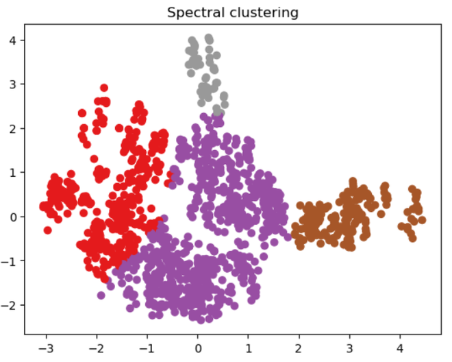
Spectral Clustering

The clustering results are visualized using matplotlib.pyplot by the code. With the reduced-dimensionality data (X_principal), it generates a two-dimensional scatter plot (P1 and P2). The spectral clustering model’s predicted cluster labels are represented by the colors of the data points. The plot is called “Spectral clustering” and plt.show() is used to display it.

Visualizing the Spectral Cluster using different Affinity

Python3

# Building the clustering model with 'polynomial' affinity
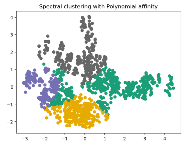
spectral_model_poly = SpectralClustering(
    n_clusters=4, affinity='poly', degree=3)

# Training the model and storing the predicted cluster labels
labels_poly = spectral_model_poly.fit_predict(X_principal)

# Visualizing the clustering with 'polynomial' affinity and a different colormap
plt.scatter(X_principal['P1'], X_principal['P2'],
            c=SpectralClustering(n_clusters=4, affinity='poly', degree=3).fit_predict(X_principal), cmap=plt.cm.Dark2)
plt.title("Spectral clustering with Polynomial affinity")
plt.show()

Output:

Advantages of Spectral clustering

1. Handling Non-Convex Clusters: Unlike traditional clustering methods like K-Means, spectral clustering can identify non-convex and irregularly shaped clusters, making it well-suited for complex datasets.
2. Hidden Structure Discovery: Spectral clustering can unveil underlying structures and patterns within data that may not be apparent using other techniques.
3. Robustness to Noise: It is relatively robust to noisy data, making it suitable for real-world datasets with imperfections.
4. Versatility: Spectral clustering is versatile and can be applied to a wide range of domains, from image processing to social network analysis.

Disadvantages of Spectral Clustering

While spectral clustering offers many advantages, it also has some limitations:

1. Sensitivity to Hyperparameters: The performance of spectral clustering can be sensitive to the choice of hyperparameters, such as the number of clusters and the affinity measure.
2. Computational Complexity: Spectral clustering can be computationally intensive, especially when dealing with large datasets.
3. Scalability: It may not scale well to extremely large datasets due to the eigenvalue decomposition step.

Conclusion

In summary, Spectral Clustering is a versatile and valuable machine learning technique that harnesses the principles of graph-based and spectral graph theory to unveil meaningful clusters within datasets. Its popularity has surged due to its competence in handling intricate data structures and uncovering concealed patterns. Spectral Clustering offers numerous advantages, such as its ability to work with non-convex clusters, reveal hidden structures, and maintain resilience against noise. It finds applications in diverse fields like image processing, social network analysis, and community detection. However, it’s crucial to acknowledge its limitations, including sensitivity to hyperparameters, computational complexity, and challenges with scalability when dealing with very large datasets. Spectral Clustering enriches the clustering toolkit, providing an effective way to unravel intricate data relationships. Its performance relies on proper parameter tuning and a firm grasp of the underlying graph theory concepts. When applied judiciously, Spectral Clustering can serve as a potent tool for unearthing concealed structures and patterns within a variety of real-world datasets.