Spectral Clustering using R

Spectral clustering is a technique used in machine learning and data analysis for grouping data points based on their similarity. The method involves transforming the data into a representation where the clusters become apparent and then using a clustering algorithm on this transformed data. In R Programming Language spectral clustering, the transformation is done using the eigenvalues and eigenvectors of a similarity matrix.

Spectral Clustering

There are some components that we used in Spectral Clustering in the R Programming Language.

Spectral clustering works by transforming the data into a lower-dimensional space where clustering is performed more effectively. The key steps involved in spectral clustering are as follows:

Affinity Matrix

Start with a dataset of data points. Compute an affinity or similarity matrix that quantifies the relationships between these data points. This matrix reflects how similar or related each pair of data points is. Common affinity measures include Gaussian similarity, k-nearest neighbors, or a user-defined similarity function.

Graph Representation

Interpret the affinity matrix as the adjacency matrix of a weighted undirected graph. In this graph, each data point corresponds to a vertex, and the weight of the edge between vertices reflects the similarity between the corresponding data points.

Laplacian Matrix

Construct the graph Laplacian matrix, which captures the connectivity of the data points in the graph. There are two main types of Laplacian matrices used in spectral clustering.

• Unnormalized Laplacian: L = D – A, where D is the degree matrix and A is the affinity matrix. The degree of a vertex is the sum of the weights of its adjacent edges.
• Normalized Laplacian: L_norm = I – D^(-1/2) * A * D^(-1/2), where D^(-1/2) is the diagonal matrix of the inverse square root of the node degrees.

Eigenvalue Decomposition

Compute the eigenvalues (λ_1, λ_2, …, λ_n) and the corresponding eigenvectors (v_1, v_2, …, v_n) of the Laplacian matrix. You typically compute a few eigenvectors, corresponding to the smallest non-zero eigenvalues.

Embedding

Use the selected eigenvectors to embed the data into a lower-dimensional space. The eigenvectors represent new features that capture the underlying structure of the data. The matrix containing these eigenvectors is referred to as the spectral embedding.

Clustering

Apply a clustering algorithm to the rows of the spectral embedding. Common clustering algorithms like k-means, normalized cuts, or spectral clustering can be used to group the data points into clusters in this lower-dimensional space.

The key idea behind spectral clustering is that by using spectral embeddings, We can potentially find clusters that are not easily separable in the original feature space. The choice of the number of clusters and the number of eigenvectors to retain in the embedding space often depends on domain knowledge, data characteristics, and application-specific requirements.

Now we will take the iris dataset for clustering.

Load the iris dataset

R

# Load the iris dataset
data(iris)

head(iris)

Output:

  Sepal.Length Sepal.Width Petal.Length Petal.Width Species Cluster
1          5.1         3.5          1.4         0.2  setosa       1
2          4.9         3.0          1.4         0.2  setosa       1
3          4.7         3.2          1.3         0.2  setosa       1
4          4.6         3.1          1.5         0.2  setosa       1
5          5.0         3.6          1.4         0.2  setosa       1
6          5.4         3.9          1.7         0.4  setosa       1

Create a Similarity Matrix

R

#Using Euclidean distance as a similarity measure
similarity_matrix <- exp(-dist(iris[, 1:4])^2 / (2 * 1^2))

#Compute Eigenvalues and Eigenvectors
eigen_result <- eigen(similarity_matrix)
eigenvalues <- eigen_result$values
eigenvectors <- eigen_result$vectors

#Choose the First k Eigenvectors
k <- 3
selected_eigenvectors <- eigenvectors[, 1:k]

#Apply K-Means Clustering
cluster_assignments <- kmeans(selected_eigenvectors, centers = k)$cluster

# Add species information to the clustering results
iris$Cluster <- factor(cluster_assignments)
iris$Species <- as.character(iris$Species)

A similarity matrix is created. This matrix quantifies the similarity between data points using the Euclidean distance as a similarity measure.

• dist(iris[, 1:4]) calculates the Euclidean distance between the data points in the first four columns of the iris dataset, which represent the sepal and petal measurements.
• exp(-dist(iris[, 1:4])^2 / (2 * 1^2)) computes a similarity value for each pair of data points. The formula used here is a Gaussian kernel, which maps distances into similarity scores.
• The eigenvalues and eigenvectors of the similarity matrix are computed using the eigen() function. Eigenvalues and eigenvectors are essential for spectral clustering.
• eigen_result$values retrieves the eigenvalues, and eigen_result$vectors retrieves the eigenvectors.
• ‘k’ is typically determined based on the number of clusters you want to find. k <- 3 indicates that you want to find three clusters.

• The kmeans() function is used to perform k-means clustering on the selected eigenvectors. It assigns data points to one of ‘k’ clusters.
• centers = k specifies that you want to find ‘k’ clusters.

• The clustering results to the iris dataset to keep track of which cluster each data point belongs to. This is stored in a new column called ‘Cluster.’
• The iris$Species column is converted to a character type using as.character(iris$Species) to ensure compatibility for visualization.

Visualize the Results

R

library(ggplot2)

# Visualizing the clusters with species names
ggplot(iris, aes(Sepal.Length, Sepal.Width, color = Cluster, label = Species)) +
  geom_point() +
  geom_text(check_overlap = TRUE, vjust = 1.5) +
  labs(title = "Spectral Clustering of Iris Dataset",
       x = "Sepal Length", y = "Sepal Width")

Output:

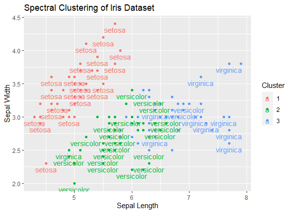
Spectral Clustering using R

ggplot(iris, aes(Sepal.Length, Sepal.Width, color = Cluster, label = Species)): This sets up the initial plot using the iris dataset. It specifies that the x-axis should represent Sepal.Length, the y-axis should represent Sepal.Width, and the color of the points should be determined by the ‘Cluster’ column. Additionally, the ‘label’ aesthetic is set to ‘Species’ to label the data points with the species names.

• geom_point(): This adds points to the plot, creating a scatterplot. Each data point represents an observation in the dataset.
• geom_text(check_overlap = TRUE, vjust = 1.5): This adds text labels to the plot, specifically the species names. The check_overlap = TRUE argument ensures that labels don’t overlap, and the vjust = 1.5 argument adjusts the vertical position of the labels for better readability.
• labs(title = “Spectral Clustering of Iris Dataset”, x = “Sepal Length”, y = “Sepal Width”): This sets the plot title and labels for the x and y axes.

Spectral Clustering with k-means

R

# Generate random data for clustering
set.seed(123)
n <- 100
k <- 3

# Create random data points with three clusters
data <- rbind(
  matrix(rnorm(n * 2, mean = c(2, 2), sd = 0.5), ncol = 2),
  matrix(rnorm(n * 2, mean = c(-2, 2), sd = 0.5), ncol = 2),
  matrix(rnorm(n * 2, mean = c(0, -2), sd = 0.5), ncol = 2)
)

# Compute the similarity matrix
similarity_matrix <- exp(-dist(data)^2)

# Perform spectral decomposition
eigen_result <- eigen(similarity_matrix)

# Extract the top-k eigenvectors
k_eigenvectors <- eigen_result$vectors[, 1:k]

# Perform k-means clustering on the eigenvectors
cluster_assignments <- kmeans(k_eigenvectors, centers = k)$cluster

# Visualize the clusters
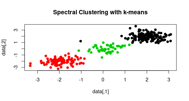
plot(data, col = cluster_assignments, pch = 19,
     main = "Spectral Clustering with k-means")

Output:

Spectral Clustering using R

First generates a random dataset with three clusters. It sets the random seed for reproducibility and creates data points using the rnorm function, which generates random numbers from a normal distribution. We stack these data points using rbind to create the dataset.

• we compute the similarity matrix, which is a measure of similarity between data points. We use the Euclidean distance to calculate the pairwise distances between data points, square these distances, and then apply the exponential function to get a similarity measure. This is a common way to compute the similarity matrix in spectral clustering.
• Spectral clustering involves the eigen-decomposition of the similarity matrix. We use the eigen function to perform the eigen-decomposition of the similarity_matrix. The result, stored in eigen_result, contains eigenvalues and eigenvectors.
• We apply the k-means clustering method to the k_eigenvectors. The k parameter specifies the number of clusters, and the resulting cluster assignments are stored in cluster_assignments.
• Finally, we visualize the clusters by plotting the data points with colors representing the cluster assignments. The col parameter is set to cluster_assignments to color the points according to their assigned clusters.

Spectral Clustering using igraph package

R

library(igraph)

# Set seed for reproducibility
set.seed(2000)

# Create a tree graph with 80 vertices and a branching factor of 4
treeGraph <- make_tree(80, children = 4, mode = "undirected")

# Generate random cluster assignments for the tree graph
num_clusters <- 4
cluster <- sample(1:num_clusters, size = vcount(treeGraph), replace = TRUE)

# Define cluster colors and labels
cluster_colors <- c("red", "blue", "green", "purple")
cluster_labels <- c("Cluster A", "Cluster B", "Cluster C", "Cluster D")

# Visualize the tree graph with markers
plot(treeGraph,
     layout = layout_nicely(treeGraph),
     vertex.size = 10,
     vertex.label = NA,
     vertex.color = cluster_colors[cluster],  # Use the defined colors
     main = "Spectral Clustering of a Tree Graph",
     edge.arrow.size = 0.2)

# Add markers to the plot legend
legend("topright", legend = cluster_labels, fill = cluster_colors,
       title = "Clusters")

Output:

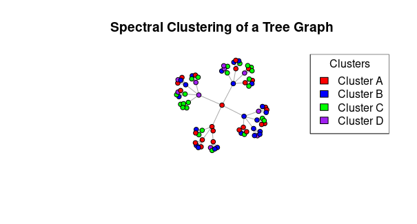
Spectral Clustering using R

First loads the igraph library, which is a package in R used for creating and analyzing network graphs and structures.

• sets the random seed to 2000 to ensure that the random number generation in the subsequent steps is reproducible. This means that if you run the code with the same seed, you will get the same results.
• a tree graph is generated using the make_tree function from the igraph package. It creates a tree graph with 80 vertices and a branching factor of 4. The mode = "undirected" parameter specifies that the graph is undirected, meaning there are no arrowheads on the edges.
• the code generates random cluster assignments for the vertices in the tree graph. num_clusters is set to 4, indicating that there are four clusters. The sample function is used to randomly assign each vertex to one of the four clusters. size = vcount(treeGraph) ensures that we generate as many cluster assignments as there are vertices in the tree graph.

We define cluster_colors and cluster_labels. cluster_colors is a vector of color names, and cluster_labels is a vector of labels corresponding to each cluster. These will be used in the plot and legend.

• layout = layout_nicely(treeGraph): Arranges the vertices in a visually pleasing layout.
• vertex.size = 10: Sets the size of the vertices to 10.
• vertex.label = NA: Removes vertex labels.
• vertex.color = cluster_colors[cluster]: Sets the vertex colors based on the cluster assignments. Each vertex is assigned a color from cluster_colors based on its cluster number.
• main = "Spectral Clustering of a Tree Graph": Sets the title of the plot.
• edge.arrow.size = 0.2: Sets the size of edge arrowheads (not applicable to this undirected graph).

Finally, this code adds a legend to the plot. It specifies the position (“topright”) of the legend, the labels (cluster_labels) for each cluster, the fill colors (cluster_colors), and a title for the legend (“Clusters”). This legend provides a visual reference to the cluster assignments and their associated colors on the graph.