Exploratory Data Analysis in Python | Set 2

In the previous article, we have discussed some basic techniques to analyze the data, now let’s see the visual techniques.

Let’s see the basic techniques –

# Loading Libraries

import numpy as np
import pandas as pd
import seaborn as sns
import matplotlib.pyplot as plt
from scipy.stats import trim_mean

# Loading Data
data = pd.read_csv("state.csv")

# Check the type of data
print ("Type : ", type(data), "\n\n")

# Printing Top 10 Records
print ("Head -- \n", data.head(10))

# Printing last 10 Records
print ("\n\n Tail -- \n", data.tail(10))

# Adding a new column with derived data
data['PopulationInMillions'] = data['Population']/1000000

# Changed data
print (data.head(5))

# Rename column heading as it
# has '.' in it which will create
# problems when dealing functions

data.rename(columns ={'Murder.Rate': 'MurderRate'},
                                    inplace = True)

# Lets check the column headings
list(data)

Output :

Type : class 'pandas.core.frame.DataFrame'


Head -- 
          State  Population  Murder.Rate Abbreviation
0      Alabama     4779736          5.7           AL
1       Alaska      710231          5.6           AK
2      Arizona     6392017          4.7           AZ
3     Arkansas     2915918          5.6           AR
4   California    37253956          4.4           CA
5     Colorado     5029196          2.8           CO
6  Connecticut     3574097          2.4           CT
7     Delaware      897934          5.8           DE
8      Florida    18801310          5.8           FL
9      Georgia     9687653          5.7           GA


 Tail -- 
             State  Population  Murder.Rate Abbreviation
40   South Dakota      814180          2.3           SD
41      Tennessee     6346105          5.7           TN
42          Texas    25145561          4.4           TX
43           Utah     2763885          2.3           UT
44        Vermont      625741          1.6           VT
45       Virginia     8001024          4.1           VA
46     Washington     6724540          2.5           WA
47  West Virginia     1852994          4.0           WV
48      Wisconsin     5686986          2.9           WI
49        Wyoming      563626          2.7           WY


        State  Population  Murder.Rate Abbreviation  PopulationInMillions
0     Alabama     4779736          5.7           AL              4.779736
1      Alaska      710231          5.6           AK              0.710231
2     Arizona     6392017          4.7           AZ              6.392017
3    Arkansas     2915918          5.6           AR              2.915918
4  California    37253956          4.4           CA             37.253956


['State', 'Population', 'MurderRate', 'Abbreviation']

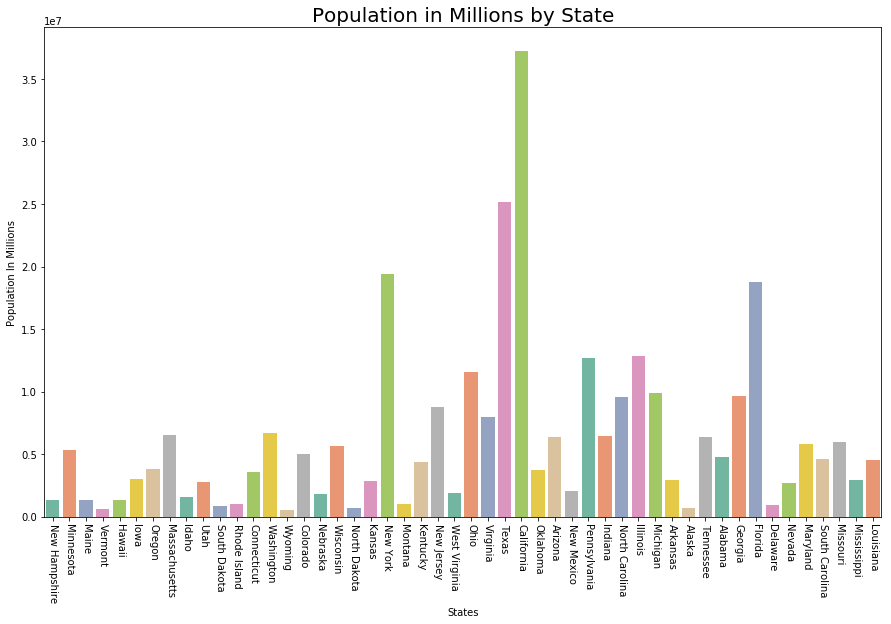
Visualizing Population per Million

# Plot Population In Millions
fig, ax1 = plt.subplots()
fig.set_size_inches(15,  9)


ax1 = sns.barplot(x ="State", y ="Population",
                  data = data.sort_values('MurderRate'),
                                        palette ="Set2")

ax1.set(xlabel ='States', ylabel ='Population In Millions')
ax1.set_title('Population in Millions by State', size = 20)

plt.xticks(rotation =-90)

Output:

(array([ 0,  1,  2,  3,  4,  5,  6,  7,  8,  9, 10, 11, 12, 13, 14, 15, 16,
        17, 18, 19, 20, 21, 22, 23, 24, 25, 26, 27, 28, 29, 30, 31, 32, 33,
        34, 35, 36, 37, 38, 39, 40, 41, 42, 43, 44, 45, 46, 47, 48, 49]),
 a list of 50 Text xticklabel objects)

Visualizing Murder Rate per Lakh

# Plot Murder Rate per 1, 00, 000

fig, ax2 = plt.subplots()
fig.set_size_inches(15,  9)


ax2 = sns.barplot(
    x ="State", y ="MurderRate",
    data = data.sort_values('MurderRate', ascending = 1),
                                         palette ="husl")

ax2.set(xlabel ='States', ylabel ='Murder Rate per 100000')
ax2.set_title('Murder Rate by State', size = 20)

plt.xticks(rotation =-90)

Output :

(array([ 0,  1,  2,  3,  4,  5,  6,  7,  8,  9, 10, 11, 12, 13, 14, 15, 16,
        17, 18, 19, 20, 21, 22, 23, 24, 25, 26, 27, 28, 29, 30, 31, 32, 33,
        34, 35, 36, 37, 38, 39, 40, 41, 42, 43, 44, 45, 46, 47, 48, 49]),
 a list of 50 Text xticklabel objects)

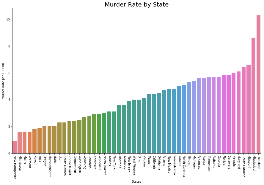
Although Louisiana is ranked 17 by population (about 4.53M), it has the highest Murder rate of 10.3 per 1M people.

Code #1 : Standard Deviation

Population_std = data.Population.std()
print ("Population std : ", Population_std)

MurderRate_std = data.MurderRate.std()
print ("\nMurderRate std : ", MurderRate_std)

Output :

Population std :  6848235.347401142

MurderRate std :  1.915736124302923

Code #2 : Variance

Population_var = data.Population.var()
print ("Population var : ", Population_var)

MurderRate_var = data.MurderRate.var()
print ("\nMurderRate var : ", MurderRate_var)

Output :

Population var :  46898327373394.445

MurderRate var :  3.670044897959184

Code #3 : Inter Quartile Range

# Inter Quartile Range of Population
population_IQR = data.Population.describe()['75 %'] -
                 data.Population.describe()['25 %']

print ("Population IQR : ", population_IRQ)

# Inter Quartile Range of Murder Rate
MurderRate_IQR = data.MurderRate.describe()['75 %'] -
                 data.MurderRate.describe()['25 %']

print ("\nMurderRate IQR : ", MurderRate_IQR)

Output :

Population IQR :  4847308.0

MurderRate IQR :  3.124999999999999

Code #4 : Median Absolute Deviation (MAD)

Population_mad = data.Population.mad()
print ("Population mad : ", Population_mad)

MurderRate_mad = data.MurderRate.mad()
print ("\nMurderRate mad : ", MurderRate_mad)

Output :

Population mad :  4450933.356000001

MurderRate mad :  1.5526400000000005