Displaying 3D images in Python

In this article, we will discuss how to display 3D images using different methods, (i.e 3d projection, view_init() method, and using a loop) in Python.

Module Needed

• Matplotlib: It is a plotting library for Python programming it serves as a visualization utility library, Matplotlib is built on NumPy arrays, and designed to work with the broader SciPy stack.
• Numpy: It is a general-purpose array-processing package. It provides a high-performance multidimensional array and matrices along with a large collection of high-level mathematical functions.
• mpl_toolkits: It provides some basic 3d plotting (scatter, surf, line, mesh) tools.

Example 1:

In this example, we created a 3d image of a scatter sin wave. Here we have created an array of points using ‘np.arrange’ and ‘np.sin’.NumPy.sin: This mathematical function helps the user to calculate trigonometric sine for all x(being the array elements), and another function is the scatter() method which is the matplotlib library used to draw a scatter plot.

Syntax: np.arrange(start, stop, step) : It returns an array with evenly spaced elements as per the interval.

Parameters:

• start: start of interval range.
• stop: end of interval range.
• step: step size of the interval.

Python3

# Import libraries
import numpy as np
import matplotlib.pyplot as plt
from mpl_toolkits.mplot3d import Axes3D

# Change the Size of Graph using
# Figsize
fig = plt.figure(figsize=(10, 10))

# Generating a 3D sine wave
ax = plt.axes(projection='3d')

# Creating array points using
# numpy
x = np.arange(0, 20, 0.1)
y = np.sin(x)
z = y*np.sin(x)
c = x + y

# To create a scatter graph
ax.scatter(x, y, z, c=c)

# turn off/on axis
plt.axis('off')

# show the graph
plt.show()

Output:

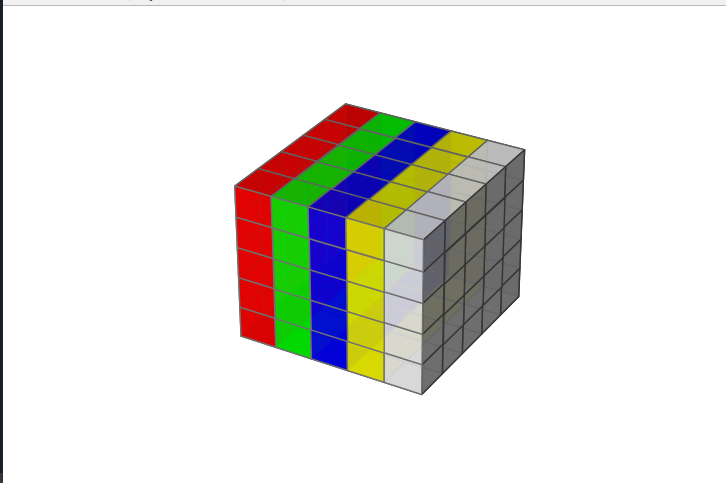
Example 2:

In this example, we are selecting the 3D axis of the dimension X =5, Y=5, Z=5, and in np.ones() we are passing the dimensions of the cube. The np.ones () function returns a new array of given shape and type, with ones.

Syntax: numpy.ones (shape, dtype = None)

After the above step, we are selecting color opacity as alpha = 0.9 ( vary from 0.0 – 1.0 ). In the next step, we are passing the dimension of axes( i.e 5, 5, 5) + number of faces for the cube ( i.e 0-4 ) in np.empty() function after that we are passing color combination and opacity for each face of the cube and in last Voxels is used to customizations of the sizes, positions, and colors. The np.empty () function return a new array of given shape and type, without initializing entries.

Syntax: numpy.empty(shape) 

Python3

# Import libraries
import matplotlib.pyplot as plt
from mpl_toolkits.mplot3d import Axes3D
import numpy as np

# Change the Size of Graph using
# Figsize
fig = plt.figure(figsize=(10, 10))

# Generating a 3D sine wave
ax = plt.axes(projection='3d')

# Create axis
axes = [5, 5, 5]

# Create Data
data = np.ones(axes)

# Control Tranperency
alpha = 0.9

# Control colour
colors = np.empty(axes + [4])

colors[0] = [1, 0, 0, alpha]  # red
colors[1] = [0, 1, 0, alpha]  # green
colors[2] = [0, 0, 1, alpha]  # blue
colors[3] = [1, 1, 0, alpha]  # yellow
colors[4] = [1, 1, 1, alpha]  # grey

# turn off/on axis
plt.axis('off')

# Voxels is used to customizations of
# the sizes, positions and colors.
ax.voxels(data, facecolors=colors, edgecolors='grey')

Output:

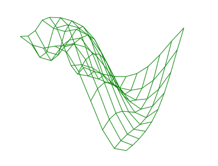
Example 3:

In this example, we use numpy.linspace() that creates an array of 10 linearly placed elements between -1 and 5, both inclusive after that the mesh grid function returns two 2-dimensional arrays, After that in order to visualize an image of 3D wireframe we require passing coordinates of X, Y, Z, color(optional).

Python3

#Import libraries
import numpy as np
import matplotlib.pyplot as plt
from mpl_toolkits.mplot3d import Axes3D

#Change the Size of Graph using Figsize
fig = plt.figure(figsize=(10,10))

#Generating a 3D sine wave
ax = plt.axes(projection='3d')


# assigning coordinates
x = np.linspace(-1, 5, 10)
y = np.linspace(-1, 5, 10)
X, Y = np.meshgrid(x, y)
Z = np.sin(np.sqrt(X ** 2 + Y ** 2))

# creating the visualization
ax.plot_wireframe(X, Y, Z, color ='green')

# turn off/on axis
plt.axis('off')

Output:

Example 4:

In this example, we plot a spiral graph, and we will see its 360-degree view using a loop. Here, view_init(elev=, azim=)This can be used to rotate the axes programmatically.‘elev’ stores the elevation angle in the z plane. ‘azim’ stores the azimuth angle in the x,y plane.D constructor. The draw() function in pyplot module of the matplotlib library is used to redraw the current figure with a pause of 0.001-time interval.

Python3

from numpy import linspace
import numpy as np
import matplotlib.pyplot as plt
from mpl_toolkits import mplot3d


# Creating 3D figure
fig = plt.figure(figsize=(8, 8))
ax = plt.axes(projection='3d')

# Creating Dataset
z = np.linspace(0, 15, 1000)
x = np.sin(z)
y = np.cos(z)
ax.plot3D(x, y, z, 'green')

# 360 Degree view
for angle in range(0, 360):
    ax.view_init(angle, 30)
    plt.draw()
    plt.pause(.001)

plt.show()

Output: