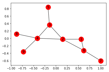
import networkx as nx
edges = [(1, 2), (1, 6), (2, 3), (2, 4), (2, 6),
(3, 4), (3, 5), (4, 8), (4, 9), (6, 7)]
G.add_edges_from(edges)
nx.draw_networkx(G, with_label = True)
print("Total number of nodes: ", int(G.number_of_nodes()))
print("Total number of edges: ", int(G.number_of_edges()))
print("List of all nodes: ", list(G.nodes()))
print("List of all edges: ", list(G.edges(data = True)))
print("Degree for all nodes: ", dict(G.degree()))
print("Total number of self-loops: ", int(G.number_of_selfloops()))
print("List of all nodes with self-loops: ",
list(G.nodes_with_selfloops()))
print("List of all nodes we can go to in a single step from node 2: ",
list(G.neighbors(2)))
|
Output:
Total number of nodes: 9
Total number of edges: 10
List of all nodes: [1, 2, 3, 4, 5, 6, 7, 8, 9]
List of all edges: [(1, 2, {}), (1, 6, {}), (2, 3, {}), (2, 4, {}), (2, 6, {}), (3, 4, {}), (3, 5, {}), (4, 8, {}), (4, 9, {}), (6, 7, {})]
Degree for all nodes: {1: 2, 2: 4, 3: 3, 4: 4, 5: 1, 6: 3, 7: 1, 8: 1, 9: 1}
Total number of self-loops: 0
List of all nodes with self-loops: []
List of all nodes we can go to in a single step from node 2: [1, 3, 4, 6]
Creating Weighted undirected Graph –
Add list of all edges along with assorted weights –
import networkx as nx
G = nx.Graph()
edges = [(1, 2, 19), (1, 6, 15), (2, 3, 6), (2, 4, 10),
(2, 6, 22), (3, 4, 51), (3, 5, 14), (4, 8, 20),
(4, 9, 42), (6, 7, 30)]
G.add_weighted_edges_from(edges)
nx.draw_networkx(G, with_labels = True)
|
We can add the edges via an Edge List, which needs to be saved in a .txt format (eg. edge_list.txt)
G = nx.read_edgelist('edge_list.txt', data =[('Weight', int)])
|
1 2 19
1 6 15
2 3 6
2 4 10
2 6 22
3 4 51
3 5 14
4 8 20
4 9 42
6 7 30
Edge list can also be read via a Pandas Dataframe –
import pandas as pd
df = pd.read_csv('edge_list.txt', delim_whitespace = True,
header = None, names =['n1', 'n2', 'weight'])
G = nx.from_pandas_dataframe(df, 'n1', 'n2', edge_attr ='weight')
print(list(G.edges(data = True)))
|
Output:
[(1, 2, {'weight': 19}),
 (1, 6, {'weight': 15}),
 (2, 3, {'weight': 6}),
 (2, 4, {'weight': 10}),
 (2, 6, {'weight': 22}),
 (3, 4, {'weight': 51}),
 (3, 5, {'weight': 14}),
 (4, 8, {'weight': 20}),
 (4, 9, {'weight': 42}),
 (6, 7, {'weight': 30})]
We would now explore the different visualization techniques of a Graph.
For this, We’ve created a Dataset of various Indian cities and the distances between them and saved it in a .txt file, edge_list.txt.
Kolkata Mumbai 2031
Mumbai Pune 155
Mumbai Goa 571
Kolkata Delhi 1492
Kolkata Bhubaneshwar 444
Mumbai Delhi 1424
Delhi Chandigarh 243
Delhi Surat 1208
Kolkata Hyderabad 1495
Hyderabad Chennai 626
Chennai Thiruvananthapuram 773
Thiruvananthapuram Hyderabad 1299
Kolkata Varanasi 679
Delhi Varanasi 821
Mumbai Bangalore 984
Chennai Bangalore 347
Hyderabad Bangalore 575
Kolkata Guwahati 1031
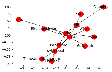
Now, we will make a Graph by the following code. We will also add a node attribute to all the cities which will be the population of each city.
import networkx as nx
G = nx.read_weighted_edgelist('edge_list.txt', delimiter =" ")
population = {
'Kolkata' : 4486679,
'Delhi' : 11007835,
'Mumbai' : 12442373,
'Guwahati' : 957352,
'Bangalore' : 8436675,
'Pune' : 3124458,
'Hyderabad' : 6809970,
'Chennai' : 4681087,
'Thiruvananthapuram' : 460468,
'Bhubaneshwar' : 837737,
'Varanasi' : 1198491,
'Surat' : 4467797,
'Goa' : 40017,
'Chandigarh' : 961587
}
for i in list(G.nodes()):
G.nodes[i]['population'] = population[i]
nx.draw_networkx(G, with_label = True)
|
Output:
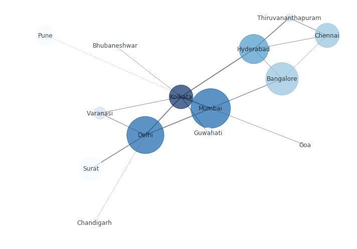
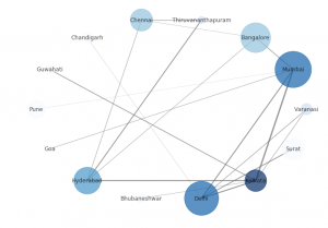
But, we can customize the Network to provide more information visually by following these steps:
- The size of the node is proportional to the population of the city.
- The intensity of colour of the node is directly proportional to the degree of the node.
- The width of the edge is directly proportional to the weight of the edge, in this case, the distance between the cities.
plt.figure(figsize =(10, 7))
node_color = [G.degree(v) for v in G]
node_size = [0.0005 * nx.get_node_attributes(G, 'population')[v] for v in G]
edge_width = [0.0015 * G[u][v]['weight'] for u, v in G.edges()]
nx.draw_networkx(G, node_size = node_size,
node_color = node_color, alpha = 0.7,
with_labels = True, width = edge_width,
edge_color ='.4', cmap = plt.cm.Blues)
plt.axis('off')
plt.tight_layout();
|
Output:
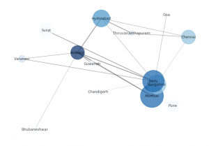
We can see in the above code, we have specified the layout type as tight. You can find the different layout techniques and try a few of them as shown in the code below:
print("The various layout options are:")
print([x for x in nx.__dir__() if x.endswith('_layout')])
node_color = [G.degree(v) for v in G]
node_size = [0.0005 * nx.get_node_attributes(G, 'population')[v] for v in G]
edge_width = [0.0015 * G[u][v]['weight'] for u, v in G.edges()]
plt.figure(figsize =(10, 9))
pos = nx.random_layout(G)
print("Random Layout:")
nx.draw_networkx(G, pos, node_size = node_size,
node_color = node_color, alpha = 0.7,
with_labels = True, width = edge_width,
edge_color ='.4', cmap = plt.cm.Blues)
plt.figure(figsize =(10, 9))
pos = nx.circular_layout(G)
print("Circular Layout")
nx.draw_networkx(G, pos, node_size = node_size,
node_color = node_color, alpha = 0.7,
with_labels = True, width = edge_width,
edge_color ='.4', cmap = plt.cm.Blues)
|
Output:
The various layout options are:
['rescale_layout',
 'random_layout',
 'shell_layout',
 'fruchterman_reingold_layout',
 'spectral_layout',
 'kamada_kawai_layout',
 'spring_layout',
 'circular_layout']

Random Layout:


Circular Layout:
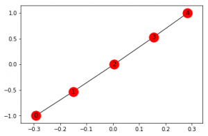
Networkx allows us to create a Path Graph, i.e. a straight line connecting a number of nodes in the following manner:
G2 = nx.path_graph(5)
nx.draw_networkx(G2, with_labels = True)
|
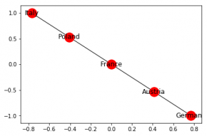
We can rename the nodes –
G2 = nx.path_graph(5)
new = {0:"Germany", 1:"Austria", 2:"France", 3:"Poland", 4:"Italy"}
G2 = nx.relabel_nodes(G2, new)
nx.draw_networkx(G2, with_labels = True)
|
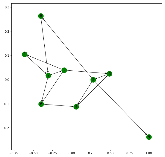
Creating Directed Graph –
Networkx allows us to work with Directed Graphs. Their creation, adding of nodes, edges etc. are exactly similar to that of an undirected graph as discussed here.
The following code shows the basic operations on a Directed graph.
import networkx as nx
G = nx.DiGraph()
G.add_edges_from([(1, 1), (1, 7), (2, 1), (2, 2), (2, 3),
(2, 6), (3, 5), (4, 3), (5, 4), (5, 8),
(5, 9), (6, 4), (7, 2), (7, 6), (8, 7)])
plt.figure(figsize =(9, 9))
nx.draw_networkx(G, with_label = True, node_color ='green')
print("Total number of nodes: ", int(G.number_of_nodes()))
print("Total number of edges: ", int(G.number_of_edges()))
print("List of all nodes: ", list(G.nodes()))
print("List of all edges: ", list(G.edges()))
print("In-degree for all nodes: ", dict(G.in_degree()))
print("Out degree for all nodes: ", dict(G.out_degree))
print("Total number of self-loops: ", int(G.number_of_selfloops()))
print("List of all nodes with self-loops: ",
list(G.nodes_with_selfloops()))
print("List of all nodes we can go to in a single step from node 2: ",
list(G.successors(2)))
print("List of all nodes from which we can go to node 2 in a single step: ",
list(G.predecessors(2)))
|
Output:
Total number of nodes: 9
Total number of edges: 15
List of all nodes: [1, 2, 3, 4, 5, 6, 7, 8, 9]
List of all edges: [(1, 1), (1, 7), (2, 1), (2, 2), (2, 3), (2, 6), (3, 5), (4, 3), (5, 8), (5, 9), (5, 4), (6, 4), (7, 2), (7, 6), (8, 7)]
In-degree for all nodes: {1: 2, 2: 2, 3: 2, 4: 2, 5: 1, 6: 2, 7: 2, 8: 1, 9: 1}
Out degree for all nodes: {1: 2, 2: 4, 3: 1, 4: 1, 5: 3, 6: 1, 7: 2, 8: 1, 9: 0}
Total number of self-loops: 2
List of all nodes with self-loops: [1, 2]
List of all nodes we can go to in a single step from node 2: [1, 2, 3, 6]
List of all nodes from which we can go to node 2 in a single step: [2, 7]
Now, we will show the basic operations for a MultiGraph. Networkx allows us to create both directed and undirected Multigraphs. A Multigraph is a Graph where multiple parallel edges can connect the same nodes.
For example, let us create a network of 10 people, A, B, C, D, E, F, G, H, I and J. They have four different relations among them namely Friend, Co-worker, Family and Neighbour. A relation between two people isn’t restricted to a single kind.
But the visualization of Multigraph in Networkx is not clear. It fails to show multiple edges separately and these edges overlap.
import networkx as nx
import matplotlib.pyplot as plt
G = nx.MultiGraph()
relations = [('A', 'B', 'neighbour'), ('A', 'B', 'friend'), ('B', 'C', 'coworker'),
('C', 'F', 'coworker'), ('C', 'F', 'friend'), ('F', 'G', 'coworker'),
('F', 'G', 'family'), ('C', 'E', 'friend'), ('E', 'D', 'family'),
('E', 'I', 'coworker'), ('E', 'I', 'neighbour'), ('I', 'J', 'coworker'),
('E', 'J', 'friend'), ('E', 'H', 'coworker')]
for i in relations:
G.add_edge(i[0], i[1], relation = i[2])
plt.figure(figsize =(9, 9))
nx.draw_networkx(G, with_label = True)
print("Total number of nodes: ", int(G.number_of_nodes()))
print("Total number of edges: ", int(G.number_of_edges()))
print("List of all nodes: ", list(G.nodes()))
print("List of all edges: ", list(G.edges(data = True)))
print("Degree for all nodes: ", dict(G.degree()))
print("Total number of self-loops: ", int(G.number_of_selfloops()))
print("List of all nodes with self-loops: ", list(G.nodes_with_selfloops()))
print("List of all nodes we can go to in a single step from node E: ",
list(G.neighbors('E")))
|
Output:
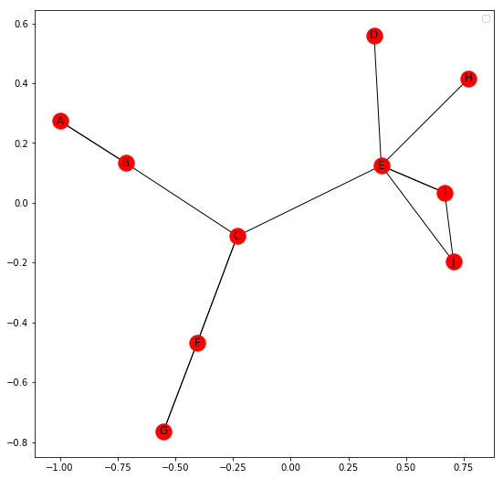
Total number of nodes: 10
Total number of edges: 14
List of all nodes: [‘E’, ‘I’, ‘D’, ‘B’, ‘C’, ‘F’, ‘H’, ‘A’, ‘J’, ‘G’]
List of all edges: [(‘E’, ‘I’, {‘relation’: ‘coworker’}), (‘E’, ‘I’, {‘relation’: ‘neighbour’}), (‘E’, ‘H’, {‘relation’: ‘coworker’}), (‘E’, ‘J’, {‘relation’: ‘friend’}), (‘E’, ‘C’, {‘relation’: ‘friend’}), (‘E’, ‘D’, {‘relation’: ‘family’}), (‘I’, ‘J’, {‘relation’: ‘coworker’}), (‘B’, ‘A’, {‘relation’: ‘neighbour’}), (‘B’, ‘A’, {‘relation’: ‘friend’}), (‘B’, ‘C’, {‘relation’: ‘coworker’}), (‘C’, ‘F’, {‘relation’: ‘coworker’}), (‘C’, ‘F’, {‘relation’: ‘friend’}), (‘F’, ‘G’, {‘relation’: ‘coworker’}), (‘F’, ‘G’, {‘relation’: ‘family’})]
Degree for all nodes: {‘E’: 6, ‘I’: 3, ‘B’: 3, ‘D’: 1, ‘F’: 4, ‘A’: 2, ‘G’: 2, ‘H’: 1, ‘J’: 2, ‘C’: 4}
Total number of self-loops: 0
List of all nodes with self-loops: []
List of all nodes we can go to in a single step from node E: [‘I’, ‘H’, ‘J’, ‘C’, ‘D’]
Similarly, a Multi Directed Graph can be created by using
Share your thoughts in the comments
Please Login to comment...