Denoising AutoEncoders In Machine Learning

Autoencoders are types of neural network architecture used for unsupervised learning. The architecture consists of an encoder and a decoder. The encoder encodes the input data into a lower dimensional space while the decode decodes the encoded data back to the original input. The network is trained to minimize the difference between decoded data and input. Autoencoders have the risk of becoming an Identify function meaning the output equals the input which makes the whole neural network of autoecoders useless. This generally happens when there are more nodes in the hidden layer than there are inputs.

Denoising Autoencoder (DAE)

Now, a denoising autoencoder is a modification of the original autoencoder in which instead of giving the original input we give a corrupted or noisy version of input to the encoder while decoder loss is calculated concerning original input only. This results in efficient learning of autoencoders and the risk of autoencoder becoming an identity function is significantly reduced.

Architecture of DAE

The denoising autoencoder (DAE) architecture resembles a standard autoencoder and consists of two main components:

Encoder:

• The encoder is a neural network with one or more hidden layers.
• It receives noisy input data instead of the original input and generates an encoding in a low-dimensional space.
• There are several ways to generate a corrupted input. The most common being adding a Gaussian noise or randomly masking some of the inputs.

Decoder:

• Similar to encoders, decoders are implemented as neural networks with one or more hidden layers.
• It takes the encoding generated by the encoder as input and reconstructs the original data.
• When calculating the Loss function it compares the output values with the original input, not with the corrupted input.

What DAE Learns?

The above architecture of using a corrupted input helps decrease the risk of overfitting and prevents the DAE from becoming an identity function.

• If DAEs are trained with partially corrupted inputs (e.g., with masking values), they learn to impute or fill in missing information during the reconstruction process. This makes them useful for tasks involving incomplete datasets.
• If DAEs are trained with partially noisy inputs (gaussian noise) DAEs tend to generalize well to unseen, real-world data with different levels of noise or corruption as they learn to extract robust features. This is beneficial in various applications where data quality is compromised, such as image denoising or signal processing.

Objective Function of DAE

The objective of DAE is to minimize the difference between the original input (clean input without the notice) and the reconstructed output. This is quantified using a reconstruction loss function. Two types of loss function are generally used depending on the type of input data.

Mean Squared Error (MSE):

If we have input image data in the form of floating pixel values i.e. values between (0 to 1) or (0 to 255) we use mse

Here,

• each of x_i is the pixel value of input data
• y_i is the pixel value of reconstructed data
  • y_i = D(E(x_i*noise) )
  • Where E represents encoder and D represents decoder
• this is summed over all the training set

Binary Cross-Entropy (log-loss):

If we have input image data in the form of bits pixel values i.e. values will be either 0 or 1 only then we can use binary cross entrop loss for each pixel value

Here

• each of xi is the pixel value of input data with value being only 0 or 1
• yi is the pixel value of reconstructed data.
  • yi = D(E(xi*noise))
• Where E represents encoder and D represents decoder
• this is summed over all the training set

Training Process of DAE

The training of DAE consists of below steps:

• Initialze ender and decoer with random weights
• Noise is intentionally added to the input data.
• Feedforward the input data through encoder and decoder to get the reconstructed image
• Calculate the reconstruction loss as defined in our objective function w
• Do backprogoagation and update weights.The goal during training is to minimize the reconstruction loss.

The training is typically done through optimization algorithms like stochastic gradient descent (SGD) or its variants.

Applications of DAE

• Image Denoising: DAEs are widely employed for cleaning and enhancing images by removing noise.
• Audio Denoising: DAEs can be applied to denoise audio signals, making them valuable in speech-enhancement tasks.
• Sensor Data Processing: DAEs are valuable in processing sensor data, removing noise, and extracting relevant information from sensor readings.
• Data Compression: Autoencoders, including DAEs, can be utilized for data compression by learning compact representations of input data.
• Feature Learning: DAEs are effective in unsupervised feature learning, capturing relevant features in the data without explicit labels.

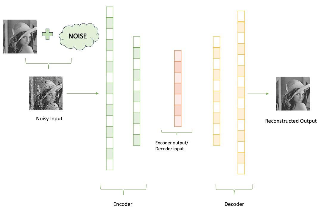
DAE architecture

Implementation of DAE

Let us implement DAE in PyTorch for MNIST dataset.

1. Import Libraries

• torch. utils.data provides tools for working with datasets and data loaders in PyTorch.
• torch-vision is a PyTorch library specifically designed for computer vision tasks. datasets contain popular datasets (like MNIST, CIFAR-10, etc.), and transforms provide image transformations and preprocessing functions.
• nn provides building blocks for constructing neural network architectures, and optim includes optimization algorithms (like SGD, Adam, etc.) for training neural networks.
• If a GPU is available, it sets the device variable to ‘cuda’; otherwise, it sets it to ‘CPU’

Python3

import torch.utils.data
from torchvision import datasets, transforms
import numpy as np
import pandas as pd

from torch import nn, optim

device = 'cuda' if torch.cuda.is_available() else 'cpu'

2. Define Dataloader

• DataLoader is used to efficiently load and iterate over batches of data during training.
• We define a transform object.
  • transforms.ToTensor(): Converts the image data into PyTorch tensors.
  • transforms.Normalize(0, 1): Normalizes the tensor values to have a mean of 0 and a standard deviation of 1.
• We then load the MNIST dataset.
  • The root parameter specifies the directory where the dataset will be stored.
  • train=True indicates that it is the training set , train = False indicates that it is the test set
  • download=True ensures that the dataset is downloaded if not already available
  • transform=transform applies the defined transform
• We have a DataLoader (train_loader and test_loader) ready to be used in your training loop.

Python3

from torch.utils.data import DataLoader

transform = transforms.Compose(
    [transforms.ToTensor(), transforms.Normalize(0, 1)])
# Load the MNIST dataset
mnist_dataset_train = datasets.MNIST(
    root='./data', train=True, download=True, transform=transform)
# Load the test MNIST dataset
mnist_dataset_test = datasets.MNIST(
    root='./data', train=False, download=True, transform=transform)

batch_size = 128
train_loader = torch.utils.data.DataLoader(
    mnist_dataset_train, batch_size=batch_size, shuffle=True)
test_loader = torch.utils.data.DataLoader(
    mnist_dataset_test, batch_size=5, shuffle=False)

3. Define our Model

• We have three fully connected layers in the encoder (fc1, fc2, fc3) and three in the decoder (fc4, fc5, fc6).
• The ReLU activation function is used for the hidden layers, and the Sigmoid activation is used for the output layer to squash the values between 0 and 1.
• Encode Method (encode):
  • The encoding method takes an input tensor x and then passes it through the encoder layers.
  • The input is noisy input .
  • The noisy input is then passed through the encoder layers (fc1, fc2, fc3), and the result is returned.
• Decode Method (decode):
  • The decode method takes the encoded representation (z) and passes it through the decoder layers (fc4, fc5, fc6).
  • The output is passed through the Sigmoid activation function to ensure values are between 0 and 1.
• Forward Method (forward):
  • The forward method defines the forward pass of the autoencoder.
  • It calls the encode method with the input tensor x, obtains the encoded representation (q), and then passes it through the decode method.
  • The final reconstructed output is returned.

Python3

class DAE(nn.Module):
    def __init__(self):
        super().__init__()

        self.fc1 = nn.Linear(784, 512)
        self.fc2 = nn.Linear(512, 256)
        self.fc3 = nn.Linear(256, 128)

        self.fc4 = nn.Linear(128, 256)
        self.fc5 = nn.Linear(256, 512)
        self.fc6 = nn.Linear(512, 784)

        self.relu = nn.ReLU()
        self.sigmoid = nn.Sigmoid()

    def encode(self, x):

        h1 = self.relu(self.fc1(x))
        h2 = self.relu(self.fc2(h1))
        return self.relu(self.fc3(h2))

    def decode(self, z):
        h4 = self.relu(self.fc4(z))
        h5 = self.relu(self.fc5(h4))
        return self.sigmoid(self.fc6(h5))

    def forward(self, x):
        q = self.encode(x.view(-1, 784))

        return self.decode(q)

4. Define our train function

We define a train function that:

• It takes an epoch number, the model, a data loader (train_loader), an optimizer, and an optional boolean cuda indicating whether to use CUDA (GPU) for training.
• Initializes a variable train_loss to keep track of the cumulative loss during training.
• Iterates over batches of data from the train_loader. Each batch consists of input data (data) and their corresponding labels (though labels are not used in this loop).
• Clears the gradients in the optimizer before the backward pass.
• Passes the input data through the autoencoder model to obtain the reconstructed output.
  • Here note that we are passing a noisy input to the encoder by adding gaussian noise
• Computes the loss between the reconstructed output (recon_batch) and the original input (data) output.
• Updates the model parameters using the optimizer.
• Prints the training progress every 100 batches.

Python3

def train(epoch, model, train_loader, optimizer,  cuda=True):
    model.train()
    train_loss = 0
    for batch_idx, (data, _) in enumerate(train_loader):
        data.to(device)
        optimizer.zero_grad()

        data_noise = torch.randn(data.shape).to(device)
        data_noise = data + data_noise

        recon_batch = model(data_noise.to(device))
        loss = criterion(recon_batch, data.view(data.size(0), -1).to(device))
        loss.backward()

        train_loss += loss.item() * len(data)
        optimizer.step()

        if batch_idx % 100 == 0:
            print('Train Epoch: {} [{}/{} ({:.0f}%)]\tLoss: {:.6f}'.format(epoch, batch_idx * len(data), len(train_loader.dataset),
                                                                           100. * batch_idx /
                                                                           len(train_loader),
                                                                           loss.item()))

    print('====> Epoch: {} Average loss: {:.4f}'.format(
        epoch, train_loss / len(train_loader.dataset)))

5. Define model, optimizer, and loss function

• We create an instance of your Denoising Autoencoder (DAE) model and move it to the specified device.
• We define Adam optimizer to optimize the model parameters. The learning rate is set to 1e-2 (0.01)
• We define Mean Squared Error (MSE) loss as the criterion. This loss measures the average squared difference between the input and target.

Python3

epochs = 10

model = DAE().to(device)
optimizer = optim.Adam(model.parameters(), lr=1e-2)
criterion = nn.MSELoss()

6. Train our model

• We train our model for the specified epochs.

Python3

for epoch in range(1, epochs + 1):
    train(epoch, model, train_loader, optimizer, True)

Output:

Train Epoch: 1 [0/60000 (0%)]    Loss: 0.232055
Train Epoch: 1 [12800/60000 (21%)]    Loss: 0.055512
Train Epoch: 1 [25600/60000 (43%)]    Loss: 0.050033
Train Epoch: 1 [38400/60000 (64%)]    Loss: 0.041521
Train Epoch: 1 [51200/60000 (85%)]    Loss: 0.043305
====> Epoch: 1 Average loss: 0.0509
Train Epoch: 2 [0/60000 (0%)]    Loss: 0.041658
Train Epoch: 2 [12800/60000 (21%)]    Loss: 0.040901
Train Epoch: 2 [25600/60000 (43%)]    Loss: 0.040894
Train Epoch: 2 [38400/60000 (64%)]    Loss: 0.039513
Train Epoch: 2 [51200/60000 (85%)]    Loss: 0.041100
====> Epoch: 2 Average loss: 0.0407
Train Epoch: 3 [0/60000 (0%)]    Loss: 0.041685
Train Epoch: 3 [12800/60000 (21%)]    Loss: 0.039040
Train Epoch: 3 [25600/60000 (43%)]    Loss: 0.038953
Train Epoch: 3 [38400/60000 (64%)]    Loss: 0.038851
Train Epoch: 3 [51200/60000 (85%)]    Loss: 0.040141

7. Performance of the model

• We use our test model to evaluate the performance of model
• Let us take 5 data samples from our test data loader add noise to it and pass it through our model.
• We will then view the output of our model and compare it with our clean data.

Python3

import matplotlib.pyplot as plt
for batch_idx, (data, labels) in enumerate(test_loader):
    data.to(device)
    optimizer.zero_grad()

    data_noise = torch.randn(data.shape).to(device)
    data_noise = data + data_noise

    recon_batch = model(data_noise.to(device))
    break


plt.figure(figsize=(20, 12))
for i in range(5):

    print(f" Image {i} with label {labels[i]}              ", end="")
    plt.subplot(3, 5, 1+i)
    plt.imshow(data_noise[i, :, :, :].view(
        28, 28).detach().numpy(), cmap='binary')
    plt.subplot(3, 5, 6+i)
    plt.imshow(recon_batch[i, :].view(28, 28).detach().numpy(), cmap='binary')
    plt.axis('off')
    plt.subplot(3, 5, 11+i)
    plt.imshow(data[i, :, :, :].view(28, 28).detach().numpy(), cmap='binary')
    plt.axis('off')
plt.show()

Output:

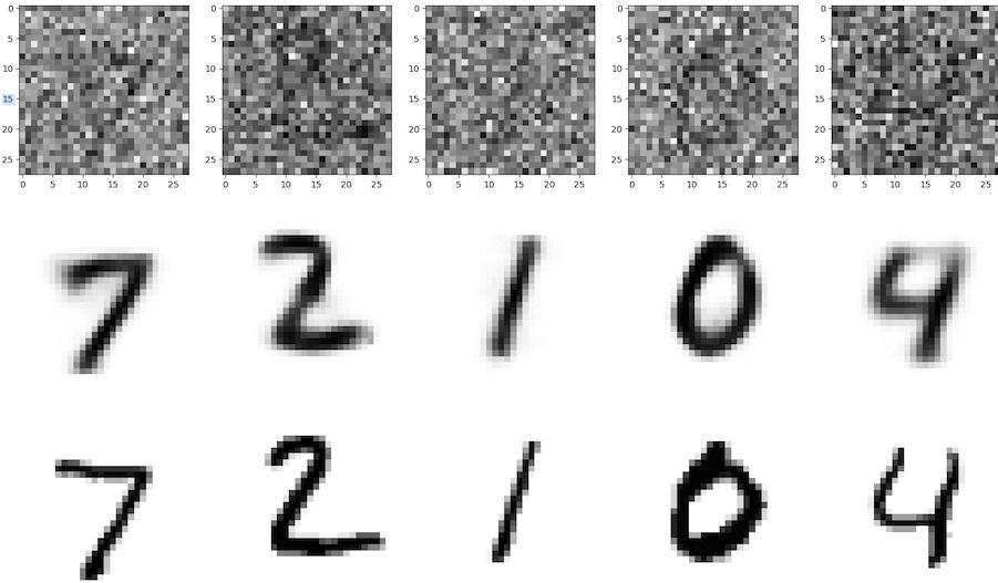
• The first row is the corrupted image
• The second row is the reconstructed image
• The last row is the actual image before addition of noise

We see that the model is able to reconstruct our original image quite well compared to our actual image with only 10 epochs of training.

Conclusion

In this article, we saw a variation of auto encoders namely denoising auto encoders, its application and its implementation in python using MNIST dataset and PyTorch framework.