How Autoencoders works ?

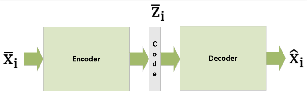
Autoencoders are the models in a dataset that find low-dimensional representations by exploiting the extreme non-linearity of neural networks. An autoencoder is made up of two parts:

Encoder – This transforms the input (high-dimensional into a code that is crisp and short.
Decoder – This transforms the shortcode into a high-dimensional input.

Assume that from a data-generating process, pdata(x), if X is a set of samples drawn. Suppose xi >>n; however, do not keep any restrictions on the support structure. An example of this is, for RGB images, xi >> n×m×3.

Here is a simple illustration of a generic autoencoder:

For a p-dimensional vector code, a parameterized function, e(•) is the definition of the encoder:

In an analogous way, the decoder is another parameterized function, d(•):

Thus, when given an input sample, xi, a full autoencoder, an amalgamated function, will provide the best alternative as output:

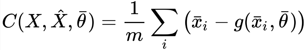
An autoencoder is trained using the back-propagation algorithm frequently based on the mean square error cost function, the reason being an autoencoder is generally applied through neural networks.

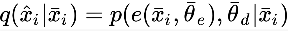
On the other hand, if you consider the process of data generation, you can look at the parameterized conditional distribution, q(•) to reiterate the objective:

This results in the cost function to develop into the Kullback-Leibler divergence between pdata(•) and q(•):

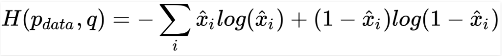
Using the optimization process, pdata can be excluded, as its entropy is constant. Now, the minimization of the cross-entropy between pdata and q and divergence is equal. The Kullback-Leibler cost function and the mean square error are equal. If you assume that pdata and q are Gaussian, you can interchange both methods of approach.

In some cases, you can implement a Bernoulli distribution for either pdata and q. But, this is only possible when you normalize the range of data to (0, 1). This is not entirely correct on a formal note though as a Bernoulli distribution is binary and xi ? {0, 1}d. The use of sigmoid output units will also result in an effective optimization for continuous samples, xi? (0, 1)d. Now, the cost function will look as follows:

Implementing a deep convolutional autoencoder –

Now let’s look at an example of a TensorFlow-based deep convolutional autoencoder. We’ll use the Olivetti faces dataset as it small in size, fits the purposes, and contains many expressions.

Step #1: Load the 400 64 × 64 grayscale image samples to prepare the set for training:

from sklearn.datasets import fetch_olivetti_faces

faces = fetch_olivetti_faces(shuffle=True, random_state=1000)
X_train = faces['images']

Step #2: Now, to increase the speed of our computation, we will resize them to 32 × 32. This will also help avoid any memory issues. We may lose a minor visual precision. Note that you can skip this if you have high computational resources.

Step #3: Let’s define the main constants.

-> number of epochs (nb_epochs)
-> batch_size
-> code_length
-> graph

import tensorflow as tf

nb_epochs = 600
batch_size = 50
code_length = 256
width = 32
height = 32

graph = tf.Graph()

Step #4: Using 50 samples per batch, we will now train the model for 600 epochs. With images size of 64 × 64 = 4, 096, we’ll get the compression ratio of 4, 096/256 = 16 times. You can always try different configurations for maximizing convergence speed and the ultimate accuracy.

Step #5: Model the encoder with these layers.

-> 2D convolution with 16 (3 × 3) filters, (2 × 2) strides, ReLU activation, and the same padding.
-> 2D convolution with 32 (3 × 3) filters, (1 × 1) strides, ReLU activation, and the same padding.
-> 2D convolution with 64 (3 × 3) filters, (1 × 1) strides, ReLU activation, and the same padding.
-> 2D convolution with 128 (3 × 3) filters, (1 × 1) strides, ReLU activation, and the same padding.

Step #6: The decoder achieves deconvolutions (a sequence of transpose convolutions).

-> 2D transpose convolution with 128 (3 × 3) filters, (2 × 2) strides, ReLU activation, and the same padding.
-> 2D transpose convolution with 64 (3 × 3) filters, (1 × 1) strides, ReLU activation, and the same padding.
-> 2D transpose convolution with 32 (3 × 3) filters, (1 × 1) strides, ReLU activation, and the same padding.
-> 2D transpose convolution with 1 (3 × 3) filter, (1 × 1) strides, Sigmoid activation, and the same padding.

The loss function is based on the L2 norm of the difference between the reconstructions and the original images. Here, Adam is the optimizer with a learning rate of α =0.001. Now, let’s look at the encoder part of the TensorFlow DAG:

import tensorflow as tf

with graph.as_default():
    input_images_xl = tf.placeholder(tf.float32,
                                     shape=(None, X_train.shape[1],
                                     X_train.shape[2], 1))

    input_images = tf.image.resize_images(input_images_xl,
                                          (width, height),
                    method=tf.image.ResizeMethod.BICUBIC)

    # Encoder
    conv_0 = tf.layers.conv2d(inputs=input_images,
                              filters=16,
                              kernel_size=(3, 3),
                              strides=(2, 2),
                              activation=tf.nn.relu,
                              padding='same')

    conv_1 = tf.layers.conv2d(inputs=conv_0,
                              filters=32,
                              kernel_size=(3, 3),
                              activation=tf.nn.relu,
                              padding='same')

    conv_2 = tf.layers.conv2d(inputs=conv_1,
                              filters=64,
                              kernel_size=(3, 3),
                              activation=tf.nn.relu,
                              padding='same')

    conv_3 = tf.layers.conv2d(inputs=conv_2,
                              filters=128,
                              kernel_size=(3, 3),
                              activation=tf.nn.relu,
                              padding='same')

The following is the coding part of the DAG:

import tensorflow as tf

with graph.as_default():

    # Code layer
    code_input = tf.layers.flatten(inputs=conv_3)

    code_layer = tf.layers.dense(inputs=code_input,
                                 units=code_length,
                                 activation=tf.nn.sigmoid)

    code_mean = tf.reduce_mean(code_layer, axis=1)

Now, let’s look at the DAG decoder:

import tensorflow as tf

with graph.as_default():

    # Decoder
    decoder_input = tf.reshape(code_layer,
                      (-1, int(width / 2),
                       int(height / 2), 1))

    convt_0 = tf.layers.conv2d_transpose(inputs=decoder_input,
                                         filters=128,
                                         kernel_size=(3, 3),
                                         strides=(2, 2),
                                         activation=tf.nn.relu,
                                         padding='same')

    convt_1 = tf.layers.conv2d_transpose(inputs=convt_0,
                                         filters=64,
                                         kernel_size=(3, 3),
                                         activation=tf.nn.relu,
                                         padding='same')

    convt_2 = tf.layers.conv2d_transpose(inputs=convt_1,
                                         filters=32,
                                         kernel_size=(3, 3),
                                         activation=tf.nn.relu,
                                         padding='same')

    convt_3 = tf.layers.conv2d_transpose(inputs=convt_2,
                                         filters=1,
                                         kernel_size=(3, 3),
                                         activation=tf.sigmoid,
                                         padding='same')

    output_images = tf.image.resize_images(convt_3, (X_train.shape[1],
                                                    X_train.shape[2]),
                                  method=tf.image.ResizeMethod.BICUBIC)

Step #7: Here’s how you define the loss function and the Adam optimizer –

import tensorflow as tf

with graph.as_default():
    # Loss
    loss = tf.nn.l2_loss(convt_3 - input_images)

    # Training step
    training_step = tf.train.AdamOptimizer(0.001).minimize(loss)

Step #8: Now that we have defined the full DAG, we can start the session and initialize all variables.

import tensorflow as tf

session = tf.InteractiveSession(graph=graph)
tf.global_variables_initializer().run()

Step #9: We can start the training process after the initialization of TensorFlow:

import numpy as np

for e in range(nb_epochs):
    np.random.shuffle(X_train)

    total_loss = 0.0
    code_means = []

    for i in range(0, X_train.shape[0] - batch_size, batch_size):
        X = np.expand_dims(X_train[i:i + batch_size, :, :],
                                axis=3).astype(np.float32)

        _, n_loss, c_mean = session.run([training_step, loss, code_mean],
                                        feed_dict={input_images_xl: X})

        total_loss += n_loss
        code_means.append(c_mean)

    print('Epoch {}) Average loss per sample: {} (Code mean: {})'.
          format(e + 1, total_loss / float(X_train.shape[0]),
          np.mean(code_means)))

Output:

Epoch 1) Average loss per sample: 11.933397521972656 (Code mean: 0.5420681238174438)
Epoch 2) Average loss per sample: 10.294102325439454 (Code mean: 0.4132006764411926)
Epoch 3) Average loss per sample: 9.917563934326171 (Code mean: 0.38105469942092896)
...
Epoch 600) Average loss per sample: 0.4635812330245972 (Code mean: 0.42368677258491516)

When the training process culminates, 0.46 (considering 32 × 32 images) is the average loss per sample and 0.42 is the mean of the codes. This proves that the encoding is relatively dense bringing the average to 0.5. Our focus is to look at sparsity during the comparison of the result.

Some sample images have resulted in the following output of the autoencoder:

When the images are upsized to 64 × 64, the quality of the reconstruction is affected partially. However, we can reduce the compression ratio and increase the code length to get better results.

How to denoise autoencoders ?
An application of autoencoders can be found helpful when it depends on the process of transformation from input to output. It is not necessarily related to autoencoder’s ability to find lower-dimensional representations.

Let’s take a look at an example where we assume X as a zero-centered dataset and a noisy version, the sample of which will have a structure as follows:

Here, the autoencoder’s focus is to remove the noisy term and bring back the original sample, xi. If we look at this from a mathematical perspective, standard and denoising autoencoders are one and the same but we need to look at the capacity needs for considering these models. As they have to recover original samples, given a corrupted input (whose features occupy a much larger sample space), the amount and dimension of layers might be larger than for a standard autoencoder.

Of course, considering the complexity, it’s impossible to have clear insight without a few tests; therefore, I strongly suggest starting with smaller models and increasing the capacity until the optimal cost function reaches a suitable value. You can use various strategies to add noise such as, corrupting the samples contained in each batch, using a noise layer as input 1 for the encoder, or using a dropout layer as input 1 for the encoder.

One of the most collective choices is to assume that the noise is Gaussian. If so, we can create homoscedastic and heteroscedastic noise. The first case has a variance that is kept constant for all components (that is, n(i) ? N(0, ?2I)), while the second case has components that have their own variance. Looking at the nature of the issue, we can choose another apt solution. But, it is preferable to implement heteroscedastic noise to improve the sturdiness of the entire system.

How to add noise to autoencoders –

We will modify our deep convolutional autoencoder so that it can manage noisy input samples. Since the DAG is almost equal, we need to include images that original and noisy.

import tensorflow as tf

with graph.as_default():
    input_images_xl = tf.placeholder(tf.float32,
                         shape=(None, X_train.shape[1],
                         X_train.shape[2], 1))
    input_noisy_images_xl = tf.placeholder(tf.float32,
                             shape=(None, X_train.shape[1],
                             X_train.shape[2], 1))

    input_images = tf.image.resize_images(input_images_xl,
                                          (width, height),
                     method=tf.image.ResizeMethod.BICUBIC)

    input_noisy_images = tf.image.resize_images(input_noisy_images_xl,
                                                      (width, height),
                                 method=tf.image.ResizeMethod.BICUBIC)

    # Encoder
    conv_0 = tf.layers.conv2d(inputs=input_noisy_images,
                              filters=16,
                              kernel_size=(3, 3),
                              strides=(2, 2),
                              activation=tf.nn.relu,
                              padding='same')

Considering the new images, we can calculate the loss function:

# Loss
loss = tf.nn.l2_loss(convt_3 - input_images)

# Training step
training_step = tf.train.AdamOptimizer(0.001).minimize(loss)

Once the standard initialization of the variables is complete, we can start the training process considering an additive noise, ni ? N(0, 0.45) (that is, ? ? 0.2):

import numpy as np

for e in range(nb_epochs):
    np.random.shuffle(X_train)

    total_loss = 0.0
    code_means = []

    for i in range(0, X_train.shape[0] - batch_size, batch_size):
        X = np.expand_dims(X_train[i:i + batch_size, :, :],
                                 axis=3).astype(np.float32)

        Xn = np.clip(X + np.random.normal(0.0, 0.2,
                     size=(batch_size, X_train.shape[1],
                     X_train.shape[2], 1)), 0.0, 1.0)

        _, n_loss, c_mean = session.run([training_step, loss, code_mean],
                                       feed_dict={ input_images_xl: X,
                                             input_noisy_images_xl: Xn })

        total_loss += n_loss
        code_means.append(c_mean)

    print('Epoch {}) Average loss per sample: {} (Code mean: {})'.
                format(e + 1, total_loss / float(X_train.shape[0]),
                                             np.mean(code_means)))

Now that we have trained the model, we use some noisy samples to test it. Here is the output of this action –

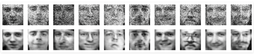
We have successfully taught the autoencoder to denoise the input images, no matter the quality of the input images. You can go ahead and try different datasets to achieve maximum noise variance.

Reference:
Hands-On Unsupervised Learning with Python.