Convolutional Variational Autoencoder in Tensorflow

In the age of Generative AI, the creation of generative models is very crucial for learning and synthesizing complex data distributions within the dataset. By incorporating convolutional layers with Variational Autoencoders, we can create a such kind of generative model. In this article, we will discuss about CVAE and implement it.

Convolutional Variational Autoencoder

A generative model which combines the strengths of convolutional neural networks and variational autoencoders. Variational Autoencoder (VAE) works as an unsupervised learning algorithm that can learn a latent representation of data by encoding it into a probabilistic distribution and then reconstructing back using the convolutional layers which enables the model to generate new, similar data points. The key working principles of a CVAE include the incorporation of convolutional layers, which are adept at capturing spatial hierarchies within data, making them particularly well-suited for image-related tasks. Additionally, CVAEs utilize variational inference, introducing probabilistic elements to the encoding-decoding process. Instead of producing a fixed latent representation, a CVAE generates a probability distribution in the latent space, enabling the model to learn not just a single deterministic representation but a range of possible representations for each input. Some of the key working principles are discussed below:

• Convolutional Layers: CVAE leverages the power of convolutional layers to efficiently capture spatial hierarchies and local patterns within images which enables the model to recognize features at different scales, providing a robust representation of the input data.
• Variational Inference: The introduction of variational inference allows CVAE to capture uncertainty in the latent space to generate a probability distribution rather than producing a single deterministic latent representation, providing a richer understanding of the data distribution and enabling the model to explore diverse latent spaces.
• Reparameterization Trick: It involves sampling from the learned latent distribution during the training process, enabling the model to backpropagate gradients effectively.

Convolutional Variational Autoencoder in Tensorflow

Import required libraries

At first, we will import all required Python libraries like NumPy, Matplotlib, TensorFlow, Keras etc. We will disable the eager execution in TensorFlow to accommodate certain operations that are executed outside the TensorFlow runtime. The TensorFlow backend session is cleared to ensure a clean slate.

Python3

import numpy as np
import matplotlib.pyplot as plt
import random
import keras
import tensorflow as tf
from keras import backend as k
from tensorflow.python.framework.ops import disable_eager_execution
disable_eager_execution()
k.clear_session()

Dataset loading and Pre-Processing

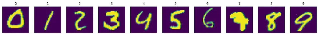
Now we will load the famous MNIST dataset and then change their datatypes to float 32. After that, we will reshape every image of the dataset in a fixed image shape (28,28,1). Then, we will define a small function (get_images_1_to_10) to select any 10 images with 0 to 9 labelling from the dataset.

Python3

# import minist dataset
(x_train, y_train), (x_test, y_test) = tf.keras.datasets.mnist.load_data()
image_shape = (28, 28, 1)
latent_dim = 2
# change datatype and reshape data
x_train = x_train.astype('float32') / 255.
x_train = x_train.reshape((x_train.shape[0],) + image_shape)
x_test = x_test.astype('float32') / 255.
x_test = x_test.reshape((x_test.shape[0],) + image_shape)

Fetch each digit images

Python3

# function to fetch 10 images of label 0 to 9
def get_images_1_to_10(x_train, y_train):
    selected_x, selected_y = [], []
    for i in range(10):
        number_index = np.where(y_train == i)[0]
        random_index = np.random.choice(len(number_index), 1, replace=False)
        select_index = number_index[random_index]
        selected_x.append(x_train[select_index[0]])
        selected_y.append(y_train[select_index][0])
    return np.array(selected_x, dtype="float32").reshape((len(selected_x),)+image_shape), np.array(selected_y, dtype="float32")


# select random 10 image of labeled 0 to 9
selected_x, selected_y = get_images_1_to_10(x_train, y_train)

Plot each digit original image

Python3

def plot_image(selected_x, selected_y, title=None, save=None):
    ncols = selected_x.shape[0]
    fig, ax = plt.subplots(nrows=1, ncols=ncols, figsize=(20, 3))
    for x, y, ax_i in zip(selected_x, selected_y, ax):
        ax_i.imshow(x.reshape((28, 28)))
        ax_i.axis("off")
        ax_i.set_title(int(y))
    if title:
        fig.suptitle(title)
    plt.show()

plot_image(selected_x, selected_y)

Output:

Convolutional Variational Autoencoder(CVAE)

As we know Autoencoders used to have three layers which are Encoding layer, bottleneck or latent space layer and decoder or output layer. In Convolutional VAE model, the encoder and decodes has two-dimensional Convolutional layers with variational layer length. So, let’s make the model layer by layer so we can gain better insights about the model structure.

Encoder Layer

• This will consist of one input layer followed by two Convolutional layers and Dense layers.

Python3

# Input
encoder_input = tf.keras.Input(shape=image_shape)
# convolutional layer 1
conv_1 = tf.keras.layers.Conv2D(
    filters=32, kernel_size=3, padding="same", activation="relu",)(encoder_input)

# convolutional layer 2
conv_2 = tf.keras.layers.Conv2D(filters=64,
                                kernel_size=3,
                                padding="same",
                                activation="relu",
                                )(conv_1)

# convolutional layer 3
conv_3 = tf.keras.layers.Conv2D(filters=64,
                                kernel_size=3,
                                padding="same",
                                activation="relu",
                                )(conv_2)
# Flatten the data
flatten = tf.keras.layers.Flatten()(conv_3)

# Dense layer 1
encoder_output = tf.keras.layers.Dense(128, activation="relu")(flatten)
z_mu = tf.keras.layers.Dense(latent_dim)(encoder_output)

# Dense layer 2
z_log_sigma = tf.keras.layers.Dense(latent_dim)(encoder_output)

• Bottleneck or Latent Layer: This is the most important layer of any type of autoencoders. Here we will define the distribution function and pass it by a Dense layer.

Python3

# sampling function for latent layer
def sampling(args):
    z_mu, z_log_sigma = args

    # epsilon in simple normal distribution
    epsilon = k.random_normal(
        shape=(k.shape(z_mu)[0], latent_dim), mean=0., stddev=1.)
    return z_mu + k.exp(z_log_sigma) * epsilon


z = tf.keras.layers.Lambda(sampling, output_shape=(
    latent_dim,))([z_mu, z_log_sigma])

Decoder Layer

• We will first define reshaping layer before transposing the convolutional layers. There are four deconvolutional layers (just transpose of Convolutional) in consideration. However, you can define most dense model for better results but adding each layer will gradually increase the model’s complexity and execution time. Also, you need more machine resources for more complex models.

Python3

# decoder layer
dense_2 = tf.keras.layers.Dense(128, activation="relu")
dense_3 = tf.keras.layers.Dense(np.prod(k.int_shape(conv_3)[1:]),
                                activation="relu"
                                )

# Reshape layer
reshape = tf.keras.layers.Reshape(k.int_shape(conv_3)[1:])

# Deconvolutional layer 1
conv_4 = tf.keras.layers.Conv2DTranspose(filters=64,
                                         kernel_size=3,
                                         padding="same",
                                         activation="relu"
                                         )
# Deconvolutional layer 2
conv_5 = tf.keras.layers.Conv2DTranspose(filters=64,
                                         kernel_size=3,
                                         padding="same",
                                         activation="relu"
                                         )

# Deconvolutional layer 3
conv_6 = tf.keras.layers.Conv2DTranspose(filters=32,
                                         kernel_size=3,
                                         padding="same",
                                         activation="relu"
                                         )

# convolutional layer 4
decoder_output = tf.keras.layers.Conv2D(filters=1,
                                        kernel_size=3,
                                        padding="same",
                                        activation="sigmoid"
                                        )

_dense_2 = dense_2(z)
_dense_3 = dense_3(_dense_2)
_reshape = reshape(_dense_3)
_conv_4 = conv_4(_reshape)
_conv_5 = conv_5(_conv_4)
_conv_6 = conv_6(_conv_5)
_decoder_output = decoder_output(_conv_6)

Defining loss function

Generally, VAE models not used to be evaluated on tradition loss functions. Most of the time there are custom and complex loss functions. However, here will use a simple custom loss function by incorporating reconstruction loss and KL loss.

• We are using binary cross entropy as the reconstruction loss.
• keras.metrics.binary_crossentropy is applied to the flatten input data x and the flattened reconstructed output z_decoded.
• KL Divergence Loss calculate how probability distribution diverges from a second.
• The formula used in the code involves mean and log-variance of the latent distribution.
• The total loss is the sum of the reconstructed loss and the KL divergence loss.

Python3

def vae_loss(x, z_decoded):
    x = k.flatten(x)
    z_decoded = k.flatten(z_decoded)

    # Reconstruction loss
    Reconstruction_loss = 786*keras.metrics.binary_crossentropy(x, z_decoded)

    # KL divergence
    kl_loss = -0.5 * k.mean(1 + z_log_sigma -
                            k.square(z_mu) - k.exp(z_log_sigma), axis=-1)
    return Reconstruction_loss + kl_loss

Visualizing model structure

CVAE models have multilayered complex structures. We have defined it layer by layer. So, before model training let’s have a look of it.

• keras.Model(encoder_input, _decoder_output) creates a model. The model combines the encoder and decoder.
• we are using RMSProp as optimizer and vae as the loss function.

Python3

cvae = keras.Model(encoder_input, _decoder_output)
cvae.compile(optimizer='rmsprop', loss=vae_loss)
cvae.summary()

Output:

Model: "model"
__________________________________________________________________________________________________
 Layer (type)                Output Shape                 Param #   Connected to                  
==================================================================================================
 input_3 (InputLayer)        [(None, 28, 28, 1)]          0         []                            
                                                                                                  
 conv2d_6 (Conv2D)           (None, 28, 28, 32)           320       ['input_3[0][0]']             
                                                                                                  
 conv2d_7 (Conv2D)           (None, 28, 28, 64)           18496     ['conv2d_6[0][0]']            
                                                                                                  
 conv2d_8 (Conv2D)           (None, 28, 28, 64)           36928     ['conv2d_7[0][0]']            
                                                                                                  
 flatten_2 (Flatten)         (None, 50176)                0         ['conv2d_8[0][0]']            
                                                                                                  
 dense_6 (Dense)             (None, 128)                  6422656   ['flatten_2[0][0]']           
                                                                                                  
 dense_7 (Dense)             (None, 2)                    258       ['dense_6[0][0]']             
                                                                                                  
 dense_8 (Dense)             (None, 2)                    258       ['dense_6[0][0]']             
                                                                                                  
 lambda (Lambda)             (None, 2)                    0         ['dense_7[0][0]',             
                                                                     'dense_8[0][0]']             
                                                                                                  
 dense_9 (Dense)             (None, 128)                  384       ['lambda[0][0]']              
                                                                                                  
 dense_10 (Dense)            (None, 50176)                6472704   ['dense_9[0][0]']             
                                                                                                  
 reshape (Reshape)           (None, 28, 28, 64)           0         ['dense_10[0][0]']            
                                                                                                  
 conv2d_transpose (Conv2DTr  (None, 28, 28, 64)           36928     ['reshape[0][0]']             
 anspose)                                                                                         
                                                                                                  
 conv2d_transpose_1 (Conv2D  (None, 28, 28, 64)           36928     ['conv2d_transpose[0][0]']    
 Transpose)                                                                                       
                                                                                                  
 conv2d_transpose_2 (Conv2D  (None, 28, 28, 32)           18464     ['conv2d_transpose_1[0][0]']  
 Transpose)                                                                                       
                                                                                                  
 conv2d_9 (Conv2D)           (None, 28, 28, 1)            289       ['conv2d_transpose_2[0][0]']  
                                                                                                  
==================================================================================================
Total params: 13044613 (49.76 MB)
Trainable params: 13044613 (49.76 MB)
Non-trainable params: 0 (0.00 Byte)
__________________________________________________________________________________________________

Train the CVAE Model

Let’s train our model with batch size 64 and four epochs. It is highly recommended to increase both on them for better results.

We will input data is used as both the input x and target y for training, this is a common in autoencoder setups where the goal is to reconstruct the input as the primary objective is to learn a compact representation of the input data also referred as latent space.

Python3

cvae.fit(x=x_train, y=x_train,
         shuffle=True,
         epochs=10,
         batch_size=64)

Output:

Train on 60000 samples
Epoch 1/10
60000/60000 [==============================] - 35s 581us/sample - loss: 180.3525
Epoch 2/10
60000/60000 [==============================] - 22s 364us/sample - loss: 149.9667
Epoch 3/10
60000/60000 [==============================] - 22s 369us/sample - loss: 145.2487
Epoch 4/10
60000/60000 [==============================] - 22s 366us/sample - loss: 142.6823
Epoch 5/10
60000/60000 [==============================] - 22s 372us/sample - loss: 141.0701
Epoch 6/10
60000/60000 [==============================] - 22s 362us/sample - loss: 139.8633
Epoch 7/10
60000/60000 [==============================] - 22s 367us/sample - loss: 138.9610
Epoch 8/10
60000/60000 [==============================] - 22s 367us/sample - loss: 138.2938
Epoch 9/10
60000/60000 [==============================] - 22s 362us/sample - loss: 137.6797
Epoch 10/10
60000/60000 [==============================] - 22s 366us/sample - loss: 137.1886
<keras.src.callbacks.History at 0x79af7fbff280>

By training the autoencoder with the same input and target data, the model learns to encode the relevant features of the input and decode them to reconstruct the original data. This is particularly useful for tasks where capturing the inherent structure and patterns in the data is the primary goal.

Artificial Digit image Generations

Model training in completed. But evaluating CVAE models are slightly different. In general case, there are various model metrics to evaluate models. But they are all are useless for CVAE. The only method of evaluation is putting original and predicted or reconstructed images side by side and visualize how clear and similar they are. However, in our custom VAE loss function the loss in low as VAE is calculated over 1000 scale. So, let keep the values aside and visualize how much clear the reconstructed images are.

Python3

# select random 10 image of labeled 0 to 9 from test dataset
test_x, test_y =  get_images_1_to_10(x_test,y_test)

gen_x = cvae.predict(test_x)

plot_image(test_x,test_y, title="Origial unique Test Digits")
plot_image(gen_x,test_y,title="Artificial Generated Digits")

Output:

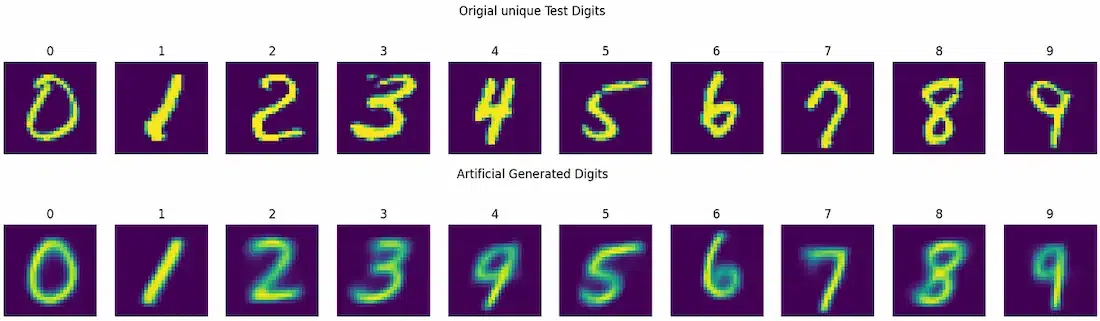
Original vs Generated Images

So, from the output we can say the model prediction is well as there is very slight difference with original images. However, for more accurate predictions we need to go for more epochs and advanced loss reduction techniques.

Benefits of using Convolutional Variational Autoencoder (CVAE)

Some of the advantages of using CVAE is listed below:

1. Image Generation: CVAE excels in generating realistic and diverse images by learning a probabilistic representation of the data distribution. It can create novel samples which retain the inherent characteristics of the training dataset.
2. Latent Space Exploration: The probabilistic nature of the latent space in CVAE allows for smooth and continuous transitions between different data points which enables meaningful exploration of the latent space, facilitating interpolation between diverse samples.
3. Uncertainty Modeling: Unlike deterministic autoencoders, CVAEs provide a measure of uncertainty in their predictions which makes them particularly valuable in applications where understanding the model’s confidence is crucial like medical image analysis or anomaly detection.
4. Robustness to Variations: CVAE is robust to variations in input data, making them suitable for tasks involving data with inherent variability like facial recognition under different lighting conditions or style transfer in images.

Conclusion

We can conclude that our CVAE model is well structed but for real-world complex datasets it is required to perform more complex and advance layering of the model and go for at least 20 epochs for better results.