Variational AutoEncoders

Autoencoders have emerged as an architecture for data representation and generation. Among them, Variational Autoencoders (VAEs) stand out, introducing probabilistic encoding and opening new avenues for diverse applications. In this article, we are going to explore the architecture and foundational concepts of variational autoencoders (VAEs).

Autoencoders are neural network architectures that are intended for the compression and reconstruction of data. It consists of an encoder and a decoder; these networks are learning a simple representation of the input data. Reconstruction loss ensures a close match of output with input, which is the basis for understanding more advanced architectures such as VAEs. The encoder aims to learn efficient data encoding from the dataset and pass it into a bottleneck architecture. The other part of the autoencoder is a decoder that uses latent space in the bottleneck layer to regenerate images similar to the dataset. These results backpropagate the neural network in the form of the loss function.

What is a Variational Autoencoder?

Variational autoencoder was proposed in 2013 by Diederik P. Kingma and Max Welling at Google and Qualcomm. A variational autoencoder (VAE) provides a probabilistic manner for describing an observation in latent space. Thus, rather than building an encoder that outputs a single value to describe each latent state attribute, we’ll formulate our encoder to describe a probability distribution for each latent attribute. It has many applications, such as data compression, synthetic data creation, etc.

Variational autoencoder is different from an autoencoder in a way that it provides a statistical manner for describing the samples of the dataset in latent space. Therefore, in the variational autoencoder, the encoder outputs a probability distribution in the bottleneck layer instead of a single output value.

Architecture of Variational Autoencoder

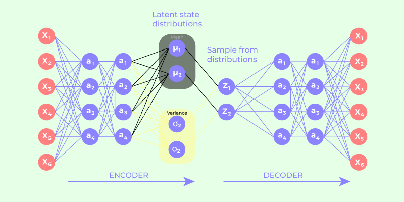
• The encoder-decoder architecture lies at the heart of Variational Autoencoders (VAEs), distinguishing them from traditional autoencoders. The encoder network takes raw input data and transforms it into a probability distribution within the latent space.
• The latent code generated by the encoder is a probabilistic encoding, allowing the VAE to express not just a single point in the latent space but a distribution of potential representations.
• The decoder network, in turn, takes a sampled point from the latent distribution and reconstructs it back into data space. During training, the model refines both the encoder and decoder parameters to minimize the reconstruction loss – the disparity between the input data and the decoded output. The goal is not just to achieve accurate reconstruction but also to regularize the latent space, ensuring that it conforms to a specified distribution.
• The process involves a delicate balance between two essential components: the reconstruction loss and the regularization term, often represented by the Kullback-Leibler divergence. The reconstruction loss compels the model to accurately reconstruct the input, while the regularization term encourages the latent space to adhere to the chosen distribution, preventing overfitting and promoting generalization.
• By iteratively adjusting these parameters during training, the VAE learns to encode input data into a meaningful latent space representation. This optimized latent code encapsulates the underlying features and structures of the data, facilitating precise reconstruction. The probabilistic nature of the latent space also enables the generation of novel samples by drawing random points from the learned distribution.

Variational Autoencoder

Mathematics behind Variational Autoencoder

Variational autoencoder uses KL-divergence as its loss function, the goal of this is to minimize the difference between a supposed distribution and original distribution of dataset.

Suppose we have a distribution z and we want to generate the observation x from it.  In other words, we want to calculate 
 We can do it by following way:

But, the calculation of p(x) can be quite difficult

 This usually makes it an intractable distribution. Hence, we need to approximate p(z|x) to q(z|x) to make it a tractable distribution. To better approximate p(z|x) to q(z|x), we will minimize the KL-divergence loss which calculates how similar two distributions are:

 By simplifying, the above minimization problem is equivalent to the following maximization problem :

 The first term represents the reconstruction likelihood and the other term ensures that our learned distribution q is similar to the true prior distribution p.

Thus our total loss consists of two terms, one is reconstruction error and other is KL-divergence loss:

Implementing Variational Autoencoder

In this implementation, we will be using the Fashion-MNIST dataset, this dataset is already available in keras.datasets API, so we don’t need to add or upload manually. You can also find the implementation in the from an.

Importing Libraries

• First, we need to import the necessary packages to our python environment. we will be using Keras package with TensorFlow as a backend.

python3

import numpy as np
import tensorflow as tf
import keras
from keras import layers

Creating a Sampling Layer

• For variational autoencoders, we need to define the architecture of two parts encoder and decoder but first, we will define the bottleneck layer of architecture, the sampling layer.

python3

# this sampling layer is the bottleneck layer of variational autoencoder,
# it uses the output from two dense layers z_mean and z_log_var as input,
# convert them into normal distribution and pass them to the decoder layer

class Sampling(layers.Layer):
    """Uses (mean, log_var) to sample z, the vector encoding a digit."""

    def call(self, inputs):
        mean, log_var = inputs
        batch = tf.shape(mean)[0]
        dim = tf.shape(mean)[1]
        epsilon = tf.random.normal(shape=(batch, dim))
        return mean + tf.exp(0.5 * log_var) * epsilon

Define Encoder Block

• Now, we define the architecture of encoder part of our autoencoder, this part takes images as input and encodes their representation in the Sampling layer.

Python3

latent_dim = 2

encoder_inputs = keras.Input(shape=(28, 28, 1))
x = layers.Conv2D(64, 3, activation="relu", strides=2, padding="same")(encoder_inputs)
x = layers.Conv2D(128, 3, activation="relu", strides=2, padding="same")(x)
x = layers.Flatten()(x)
x = layers.Dense(16, activation="relu")(x)
mean = layers.Dense(latent_dim, name="mean")(x)
log_var = layers.Dense(latent_dim, name="log_var")(x)
z = Sampling()([mean, log_var])
encoder = keras.Model(encoder_inputs, [mean, log_var, z], name="encoder")
encoder.summary()

Output:

Model: "encoder"
__________________________________________________________________________________________________
 Layer (type)                Output Shape                 Param #   Connected to                  
==================================================================================================
 input_9 (InputLayer)        [(None, 28, 28, 1)]          0         []                            
                                                                                                  
 conv2d_8 (Conv2D)           (None, 14, 14, 64)           640       ['input_9[0][0]']             
                                                                                                  
 conv2d_9 (Conv2D)           (None, 7, 7, 128)            73856     ['conv2d_8[0][0]']            
                                                                                                  
 flatten_4 (Flatten)         (None, 6272)                 0         ['conv2d_9[0][0]']            
                                                                                                  
 dense_8 (Dense)             (None, 16)                   100368    ['flatten_4[0][0]']           
                                                                                                  
 mean (Dense)                (None, 2)                    34        ['dense_8[0][0]']             
                                                                                                  
 log_var (Dense)             (None, 2)                    34        ['dense_8[0][0]']             
                                                                                                  
 sampling_4 (Sampling)       (None, 2)                    0         ['mean[0][0]',                
                                                                     'log_var[0][0]']             
                                                                                                  
==================================================================================================
Total params: 174932 (683.33 KB)
Trainable params: 174932 (683.33 KB)
Non-trainable params: 0 (0.00 Byte)
__________________________________________________________________________________________________

Define Decoder Block

• Now, we define the architecture of decoder part of our autoencoder, this part takes the output of the sampling layer as input and output an image of size (28, 28, 1) .

python3

latent_inputs = keras.Input(shape=(latent_dim,))
x = layers.Dense(7 * 7 * 64, activation="relu")(latent_inputs)
x = layers.Reshape((7, 7, 64))(x)
x = layers.Conv2DTranspose(128, 3, activation="relu", strides=2, padding="same")(x)
x = layers.Conv2DTranspose(64, 3, activation="relu", strides=2, padding="same")(x)
decoder_outputs = layers.Conv2DTranspose(1, 3, activation="sigmoid", padding="same")(x)
decoder = keras.Model(latent_inputs, decoder_outputs, name="decoder")
decoder.summary()

Output:

Model: "decoder"
_________________________________________________________________
 Layer (type)                Output Shape              Param #   
=================================================================
 input_10 (InputLayer)       [(None, 2)]               0         
                                                                 
 dense_9 (Dense)             (None, 3136)              9408      
                                                                 
 reshape_4 (Reshape)         (None, 7, 7, 64)          0         
                                                                 
 conv2d_transpose_12 (Conv2  (None, 14, 14, 128)       73856     
 DTranspose)                                                     
                                                                 
 conv2d_transpose_13 (Conv2  (None, 28, 28, 64)        73792     
 DTranspose)                                                     
                                                                 
 conv2d_transpose_14 (Conv2  (None, 28, 28, 1)         577       
 DTranspose)                                                     
                                                                 
=================================================================
Total params: 157633 (615.75 KB)
Trainable params: 157633 (615.75 KB)
Non-trainable params: 0 (0.00 Byte)
_________________________________________________________________

Define the VAE Model

• In this step, we combine the model and define the training procedure with loss functions.

python3

class VAE(keras.Model):
    def __init__(self, encoder, decoder, **kwargs):
        super().__init__(**kwargs)
        self.encoder = encoder
        self.decoder = decoder
        self.total_loss_tracker = keras.metrics.Mean(name="total_loss")
        self.reconstruction_loss_tracker = keras.metrics.Mean(
            name="reconstruction_loss"
        )
        self.kl_loss_tracker = keras.metrics.Mean(name="kl_loss")

    @property
    def metrics(self):
        return [
            self.total_loss_tracker,
            self.reconstruction_loss_tracker,
            self.kl_loss_tracker,
        ]

    def train_step(self, data):
        with tf.GradientTape() as tape:
            mean,log_var, z = self.encoder(data)
            reconstruction = self.decoder(z)
            reconstruction_loss = tf.reduce_mean(
                tf.reduce_sum(
                    keras.losses.binary_crossentropy(data, reconstruction),
                    axis=(1, 2),
                )
            )
            kl_loss = -0.5 * (1 + log_var - tf.square(mean) - tf.exp(log_var))
            kl_loss = tf.reduce_mean(tf.reduce_sum(kl_loss, axis=1))
            total_loss = reconstruction_loss + kl_loss
        grads = tape.gradient(total_loss, self.trainable_weights)
        self.optimizer.apply_gradients(zip(grads, self.trainable_weights))
        self.total_loss_tracker.update_state(total_loss)
        self.reconstruction_loss_tracker.update_state(reconstruction_loss)
        self.kl_loss_tracker.update_state(kl_loss)
        return {
            "loss": self.total_loss_tracker.result(),
            "reconstruction_loss": self.reconstruction_loss_tracker.result(),
            "kl_loss": self.kl_loss_tracker.result(),
        }

Train the VAE

• Now it’s the right time to train our variational autoencoder model, we will train it for 10 epochs.  But first we need to import the fashion MNIST dataset.

python3

(x_train, _), (x_test, _) = keras.datasets.fashion_mnist.load_data()
fashion_mnist = np.concatenate([x_train, x_test], axis=0)
fashion_mnist = np.expand_dims(fashion_mnist, -1).astype("float32") / 255

vae = VAE(encoder, decoder)
vae.compile(optimizer=keras.optimizers.Adam())
vae.fit(fashion_mnist, epochs=10, batch_size=128)

Output:

Epoch 1/10
547/547 [==============================] - 12s 15ms/step - loss: 279.0265 - reconstruction_loss: 265.4565 - kl_loss: 7.4453
Epoch 2/10
547/547 [==============================] - 9s 16ms/step - loss: 270.6755 - reconstruction_loss: 262.7192 - kl_loss: 7.3106
Epoch 3/10
547/547 [==============================] - 8s 15ms/step - loss: 268.7467 - reconstruction_loss: 261.6213 - kl_loss: 7.2532
Epoch 4/10
547/547 [==============================] - 9s 17ms/step - loss: 268.4030 - reconstruction_loss: 260.6729 - kl_loss: 7.1995
Epoch 5/10
547/547 [==============================] - 9s 16ms/step - loss: 267.5622 - reconstruction_loss: 260.0038 - kl_loss: 7.1871
Epoch 6/10
547/547 [==============================] - 8s 15ms/step - loss: 266.9597 - reconstruction_loss: 259.2417 - kl_loss: 7.1737
Epoch 7/10
547/547 [==============================] - 8s 15ms/step - loss: 266.0508 - reconstruction_loss: 258.7231 - kl_loss: 7.1072
Epoch 8/10
547/547 [==============================] - 8s 15ms/step - loss: 265.1775 - reconstruction_loss: 258.2050 - kl_loss: 7.0736
Epoch 9/10
547/547 [==============================] - 8s 16ms/step - loss: 264.4663 - reconstruction_loss: 257.8303 - kl_loss: 7.0655
Epoch 10/10
547/547 [==============================] - 8s 15ms/step - loss: 264.6552 - reconstruction_loss: 257.3342 - kl_loss: 7.0278
<keras.src.callbacks.History at 0x785cc25dd540>

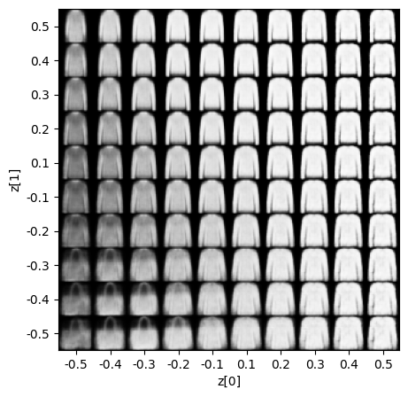
Display Sampled Images

• In this step, we display training results, we will be displaying these results according to their values in latent space vectors.

python3

import matplotlib.pyplot as plt

def plot_latent_space(vae, n=10, figsize=5):
    # display a n*n 2D manifold of images
    img_size = 28
    scale = 0.5
    figure = np.zeros((img_size * n, img_size * n))
    # linearly spaced coordinates corresponding to the 2D plot
    # of images classes in the latent space
    grid_x = np.linspace(-scale, scale, n)
    grid_y = np.linspace(-scale, scale, n)[::-1]

    for i, yi in enumerate(grid_y):
        for j, xi in enumerate(grid_x):
            sample = np.array([[xi, yi]])
            x_decoded = vae.decoder.predict(sample, verbose=0)
            images = x_decoded[0].reshape(img_size, img_size)
            figure[
                i * img_size : (i + 1) * img_size,
                j * img_size : (j + 1) * img_size,
            ] = images

    plt.figure(figsize=(figsize, figsize))
    start_range = img_size // 2
    end_range = n * img_size + start_range
    pixel_range = np.arange(start_range, end_range, img_size)
    sample_range_x = np.round(grid_x, 1)
    sample_range_y = np.round(grid_y, 1)
    plt.xticks(pixel_range, sample_range_x)
    plt.yticks(pixel_range, sample_range_y)
    plt.xlabel("z[0]")
    plt.ylabel("z[1]")
    plt.imshow(figure, cmap="Greys_r")
    plt.show()


plot_latent_space(vae)

Output:

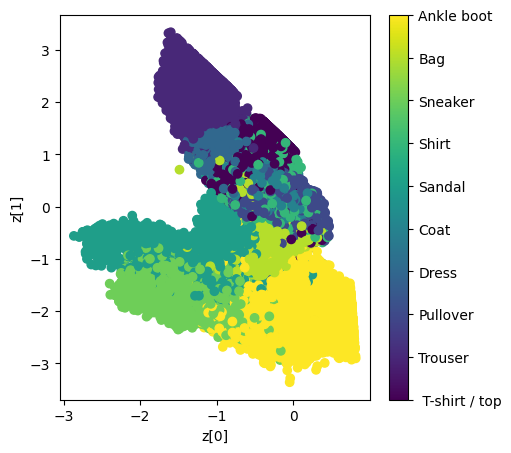
Display Latent Space Clusters

• To get a more clear view of our representational latent vectors values, we will be plotting the scatter plot of training data on the basis of their values of corresponding latent dimensions generated from the encoder .

python3

def plot_label_clusters(encoder, decoder, data, test_lab):
    z_mean, _, _ = encoder.predict(data)
    plt.figure(figsize =(12, 10))
    sc = plt.scatter(z_mean[:, 0], z_mean[:, 1], c = test_lab)
    cbar = plt.colorbar(sc, ticks = range(10))
    cbar.ax.set_yticklabels([labels.get(i) for i in range(10)])
    plt.xlabel("z[0]")
    plt.ylabel("z[1]")
    plt.show()


labels = {0    :"T-shirt / top",
1:    "Trouser",
2:    "Pullover",
3:    "Dress",
4:    "Coat",
5:    "Sandal",
6:    "Shirt",
7:    "Sneaker",
8:    "Bag",
9:    "Ankle boot"}

(x_train, y_train), _ = keras.datasets.fashion_mnist.load_data()
x_train = np.expand_dims(x_train, -1).astype("float32") / 255
plot_label_clusters(encoder, decoder, x_train, y_train)

Output:

Conclusion

In conclusion, this article has delved into the architecture and foundational concepts of Variational Autoencoders (VAEs), shedding light on their probabilistic encoding approach and applications. The article introduced autoencoders as neural networks for data compression and reconstruction, paving the way for a deeper understanding of VAEs.

The implementation section provided a practical guide using the Fashion-MNIST dataset, utilizing Keras with TensorFlow. The code showcased the definition of the encoder, decoder, and sampling layers, culminating in the creation of the VAE model. Training results, including loss values and a scatter plot for latent space visualization, were presented to provide insights into the model’s performance.

Frequently Asked Questions (FAQs)

1. What is the difference between variational and standard autoencoder?

Variational autoencoders introduce a probabilistic interpretation in the latent space, allowing for the generation of diverse outputs by sampling from learned distributions. This contrasts with standard autoencoders, which use a deterministic mapping in the latent space.

2. What are the uses of VAEs?

VAE have various applications due to their ability to model complex probability distributions like – image generation, data generation, anomaly detection, data imputation, and more.

3. What is the difference between PCA and Variational autoencoder?

PCA focuses on finding the principal components to represent existing data in a lower-dimensional space, while VAEs learn probabilistic mapping that allows for generating new data points.

4. What is the drawback of VAE?

VAEs has a drawback of generating blurry reconstructions and unrealistic outputs.

5. What is better GANs or VAE?

For image generation GANs is a better option as it generates high quality samples and VAE is a better option to use in signal analysis.