Comparison of Manifold Learning methods in Scikit Learn

In machine learning, manifold learning is crucial in order to overcome the challenges posed by high-dimensional and non-linear data. Reducing the amount of features in a dataset is done using the dimensionality reduction technique.  When working with high-dimensional data, where each data point has a number of properties, it is extremely useful. A dimensionality reduction technique called manifold learning can be used to see high-dimensional data in lower-dimensional spaces. It is especially effective when the data is non-linear in nature.

Scikit-Learn is a popular Python machine-learning package that includes a variety of learning techniques for reducing data dimensionality.

Manifold Learning

Manifold learning is a technique for dimensionality reduction used in machine learning that seeks to preserve the underlying structure of high-dimensional data while representing it in a lower-dimensional environment. This technique is particularly useful when the data has a non-linear structure that cannot be adequately captured by linear approaches like Principal Component Analysis (PCA).

Features of Manifold Learning

• Capturing the complex linkages and non-linear relationships in the data, 
• provides a better representation for upcoming analysis. 
• Makes feature extraction easier, identifies important patterns, and reduces noise. 
• Boost the effectiveness of machine learning algorithms by keeping the data’s natural structure. 
• Provide more accurate modeling and forecasting, which is especially helpful when dealing with data that linear techniques are unable to fully model.

In this post, we will examine four manifold learning algorithms that are as follows:

• t-Distributed Stochastic Neighbor Embedding(t-SNE)
• Isomap
• Locally Linear Embedding (LLE)
• Multi-Dimensional Scaling(MDS)

We will utilize the scikit-learn digits dataset, which contains pictures of digits (0-9) encoded as 8×8 pixel arrays. Each picture includes 64 characteristics that indicate the pixel intensity.

Steps:

1. Load the dataset and import the necessary libraries.
2. Make an instance of the manifold learning algorithm.
3. Fit the algorithm to the dataset.
4. Convert the dataset to a lower-dimensional space.
5. Visualize the converted data.

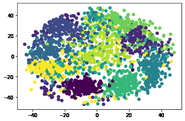
Example 1: t-SNE (t-distributed Stochastic Neighbor Embedding)

t-SNE is an effective method for displaying high-dimensional data. It is very helpful for constructing 2D or 3D representations of complicated data. t-SNE is based on the concept of probability distributions, and it attempts to minimize the divergence between two probability distributions, one measuring pairwise similarities between data points in high-dimensional space and the other measuring pairwise similarities between data points in low-dimensional space. t-SNE produces a 2D or 3D display of the data.

Python3

from sklearn.datasets import load_digits
from sklearn.manifold import TSNE
import matplotlib.pyplot as plt

digits = load_digits()
X = digits.data
y = digits.target

tsne = TSNE(n_components=2, random_state=42)
X_tsne = tsne.fit_transform(X)

plt.scatter(X_tsne[:, 0], X_tsne[:, 1], c=y)
plt.show()

Output:

t-SNE

Example 2: Isomap (Isometric Mapping)

Isomap is a dimensionality reduction approach based on the idea of geodesic distance. While mapping data points from a higher-dimensional space to a lower-dimensional space, Isomap attempts to retain the geodesic distance between them. When working with non-linear data structures, isomap comes in handy.

Python3

from sklearn.datasets import load_digits
from sklearn.manifold import Isomap
import matplotlib.pyplot as plt

digits = load_digits()
X = digits.data
y = digits.target

isomap = Isomap(n_components=2)
X_isomap = isomap.fit_transform(X)

plt.scatter(X_isomap[:, 0], X_isomap[:, 1], c=y)
plt.show()

Output:

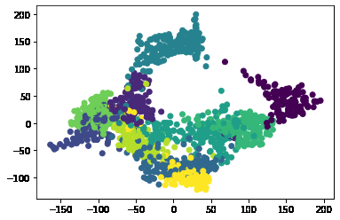
Isomap

Example 3: LLE (Locally Linear Embedding)

LLE is a dimensionality reduction approach that is built on the idea of preserving the data’s local structure. LLE attempts to find a lower-dimensional representation of the data that retains the data points’ local associations. When working with non-linear data structures, LLE is especially beneficial.

Python3

from sklearn.datasets import load_digits
from sklearn.manifold import LocallyLinearEmbedding
import matplotlib.pyplot as plt

digits = load_digits()
X = digits.data
y = digits.target

lle = LocallyLinearEmbedding(n_components=2, random_state=42)
X_lle = lle.fit_transform(X)

plt.scatter(X_lle[:, 0], X_lle[:, 1], c=y)
plt.show()

Output:

Locally Linear Embedding

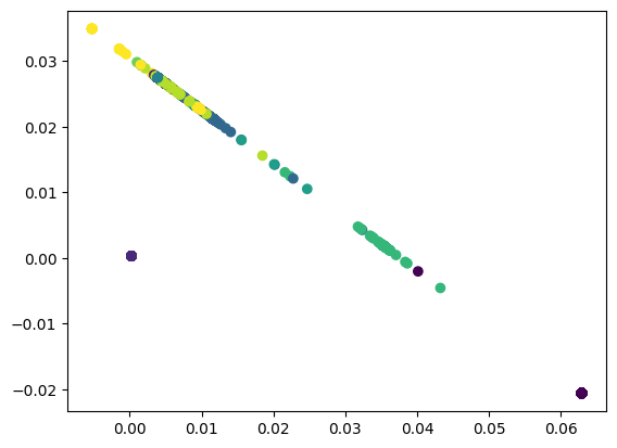
Example 4: MDS (Multi-Dimensional Scaling)

MDS is a dimensionality reduction approach that is based on the idea of maintaining the pairwise distances between data points. MDS seeks a lower-dimensional representation of the data that retains pairwise distances between data points. MDS is very helpful when working with linear data structures.

Python3

from sklearn.datasets import load_digits
from sklearn.manifold import MDS
import matplotlib.pyplot as plt

digits = load_digits()
X = digits.data
y = digits.target

mds = MDS(n_components=2, random_state=42)
X_mds = mds.fit_transform(X)

plt.scatter(X_mds[:, 0], X_mds[:, 1], c=y)
plt.show()

Output:

Multi-Dimensional Scaling