ML | T-distributed Stochastic Neighbor Embedding (t-SNE) Algorithm

T-distributed Stochastic Neighbor Embedding (t-SNE) is a nonlinear dimensionality reduction technique well-suited for embedding high-dimensional data for visualization in a low-dimensional space of two or three dimensions.

What is Dimensionality Reduction?

Dimensionality Reduction represents n-dimensions data(multidimensional data with many features) in 2 or 3 dimensions. An example of dimensionality reduction can be discussed as a classification problem i.e. student will play football or not that relies on both temperature and humidity can be collapsed into just one underlying feature since both features are correlated to a high degree. Hence, we can reduce the number of features in such problems. A 3-D classification problem can be hard to visualize, whereas a 2-D one can be mapped to simple 2-dimensional space and a 1-D problem to a simple line.

What is t-SNE Algorithm?

t-Distributed Stochastic Neighbor Embedding is a dimensionality reduction. This algorithm uses some randomized approach to reduce the dimensionality of the dataset at hand non-linearly. This focuses more on retaining the local structure of the dataset in the lower dimension as well.

This helps us explore high dimensional data as well by mapping it into lower dimensionss as the local structures are retained in the dataset we can get a feel of the same by ploting it and visualizing it in the 2D or may be 3D plane.

What is the difference between PCA and t-SNE algorithm?

Even though PCA and t-SNE both are unsupervised algorithms that are used to reduce the dimensionality of the dataset. PCA is a deterministic algorithm to reduce the dimensionality of the algorithm and the t-SNE algorithm a randomized non-linear method to map the high dimensional data to the lower dimensional. The data that is obtained after reducing the dimensionality via the t-SNE algorithm is generally used for visualization purpose only.

One more thing that we can say is an advantage of using the t-SNE data is that it is not effected by the outliers but the PCA algorithm is highly affected by the outliers because the methodologies that are used in the two algorithms is different. While we try to preserve the variance in the data using PCA algorithm we use t-SNE algorithm to retain teh local structure of the dataset.

How does t-SNE work?

t-SNE a non-linear dimensionality reduction algorithm finds patterns in the data based on the similarity of data points with features, the similarity of points is calculated as the conditional probability that point A would choose point B as its neighborr. 

It then tries to minimize the difference between these conditional probabilities (or similarities) in higher-dimensional and lower-dimensional space for a perfect representation of data points in lower-dimensional space. 

Space and Time Complexity

The algorithm computes pairwise conditional probabilities and tries to minimize the sum of the difference of the probabilities in higher and lower dimensions. This involves a lot of calculations and computations. So the algorithm takes a lot of time and space to compute. t-SNE has a quadratic time and space complexity in the number of data points.

Python Code Implementation of t-SNE on MNIST Dataset

Now let’s use the sklearn implementation of the t-SNE algorithm on the MNIST dataset which contains 10 classes that are for the 10 different digits in the mathematics.

Python3

# Importing Necessary Modules.
import numpy as np
import pandas as pd
import matplotlib.pyplot as plt
from sklearn.manifold import TSNE
from sklearn.preprocessing import StandardScaler

Now let’s load the MNIST dataset into pandas dataframe. You can download this dataset from here.

Python3

# Reading the data using pandas
df = pd.read_csv('mnist_train.csv')

# print first five rows of df
print(df.head(4))

# save the labels into a variable l.
l = df['label']

# Drop the label feature and
# store the pixel data in d.
d = df.drop("label", axis=1)

Output: 

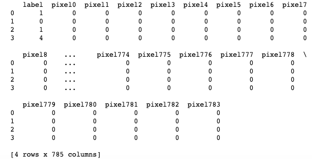
First five rows of the MNIST dataset

Before applying the t-SNE algorithm on the dataset we must standardize the data. As we know that the t-SNE algorithm is a complex algorithm which utilizes some comples non-linear methodologies to map the high dimensional data the lower dimensional it help us save some of the time complexity that will be needed to complete the process of reduction.

Python3

# Data-preprocessing: Standardizing the data
from sklearn.preprocessing import StandardScaler

standardized_data = StandardScaler().fit_transform(data)
print(standardized_data.shape)

Output:

(42000, 784)

Now let’s reduce the 784 columns data to 2 dimensions so, that we can create a scatter plot to visualize the same.

Python3

# Picking the top 1000 points as TSNE
# takes a lot of time for 15K points
data_1000 = standardized_data[0:1000, :]
labels_1000 = labels[0:1000]

model = TSNE(n_components = 2, random_state = 0)
# configuring the parameters
# the number of components = 2
# default perplexity = 30
# default learning rate = 200
# default Maximum number of iterations
# for the optimization = 1000

tsne_data = model.fit_transform(data_1000)

# creating a new data frame which
# help us in plotting the result data
tsne_data = np.vstack((tsne_data.T, labels_1000)).T
tsne_df = pd.DataFrame(data = tsne_data,
     columns =("Dim_1", "Dim_2", "label"))

# Plotting the result of tsne
sn.scatterplot(data=tsne_df, x='Dim_1', y='Dim_2',
               hue='label', palette="bright")
plt.show()

Output: 

MNIST data mapped to the 2D plane