Multinomial Naive Bayes

Multinomial Naive Bayes (MNB) is a very popular and efficient machine learning algorithm that is based on Bayes’ theorem. It is commonly used for text classification tasks where we need to deal with discrete data like word counts in documents. In this article, we will discuss MNB and implement it.

What is Multinomial Naive Bayes?

Naive Bayes is a probabilistic algorithm family based on Bayes’ Theorem. It’s “naive” because it presupposes feature independence, which means that the presence of one feature does not affect the presence of another (which may not be true in practice).

Multinomial Naive Bayes is a probabilistic classifier to calculate the probability distribution of text data, which makes it well-suited for data with features that represent discrete frequencies or counts of events in various natural language processing (NLP) tasks.

Multinomial Distribution

The term “multinomial” refers to the type of data distribution assumed by the model. The features in text classification are typically word counts or term frequencies. The multinomial distribution is used to estimate the likelihood of seeing a specific set of word counts in a document.

The probability mass function (PMF) of the Multinomial distribution is used to model the likelihood of observing a specific set of word counts in a document. It is given by:

here,

• is the total number of words in documents of class c.
• is the count of word i in document D.
• is the probability of word i occurring in a document of class c.

Let’s understand Multinomial Naive Bayes with text classification. Suppose, we have to classify a document as either to class ‘Spam’ or ‘Not Spam’ and vocabulary contains 3 words: {buy, now, free} and to classify a new document with the word counts.

The notations are provided below:

• c: Class (Spam or Not Spam)
• D: Document
• : Word in the vocabulary
• : Count of the word in the document D
• : Total number of words in documents of class c
• : Probability of word occurring the document of class c

Suppose in the training data, we have the following counts for each word in each class:

Class	buy	now	free	Total Words
Spam	20	5	10	35
Not Spam	5	15	5	25

The MLE estimate of is calculated as:

here,

• is the number of times word i appears in the document of class C
• The “+1” term is for additive smoothing (Laplace Smoothing), which helps handle the issue of zero probabilities for unseen words.

We have calculated the probabilities of each word given the class, Maximum Likelihood Estimation (MLE) for :

MLE for word ‘buy’

\theta _{Not_Spam, Buy} = \frac{5+1}{25+3} = \frac{6}{28}

Similarly, calculate MLE for for other words.

Classification of a New Document

Now let’s classify the new document with word counts {buy:1, now:0, free: 2}

When, we classify a new document, the likelihood of the document given a class is calculated using the product of these individual word probabilities:

• Likelihood calculation:
  • 
  • 

The likelihood term is then used in conjunction with prior probabilities in the Naive Bayes formula to determine the posterior probability of the class given the document:

• Applying Bayes’ theorem to calculate the posterior of each class:
  • 
  • 

After comparing the posterior probabilities and we classify the document into the class with the higher probability.

How Multinomial Naive Bayes differs from Gaussian Naive Bayes?

The Multinomial NB and Gaussian NB both are the variants of same algorithm. However they have several number of differences which are discussed below:

Multinomial Naive Bayes	Gaussian Naive Bayes
It specially designed for discrete data, particularly text data.	It is suitable for continuous data where features are real-valued and follow a Gaussian distribution.
It assumes features represent counts or frequencies of events (like word counts).	It assumes a Gaussian distribution for the likelihood.
It is commonly used in NLP for document classification tasks.	Less commonly used in text classification tasks because it’s not well-suited for count-based, discrete features.

Benefits of using Multinomial Naive Bayes

There are several benefits of using Multinomial Naive Bayes which are discussed below:

1. Efficiency: Multinomial NB is computationally efficient and can handle large datasets with many features which makes it a practical choice for text classification tasks like spam detection, sentiment analysis and document categorization where features are often count-based.
2. Easy Implementation: Multinomial NB is straightforward to implement and requires minimal hyperparameter tuning which makes it accessible for beginners and quick to deploy.
3. Robust to Irrelevant Features: The “naive” assumption of conditional independence can make Multinomial NB robust to irrelevant features or noise in the data.
4. Interpretable Results: The probabilities produced by MNB can provide insight into the likelihood of a document belonging to a specific class. It can serve as a solid baseline model for text classification tasks, against which more complex models can be compared.

Step-by-step implementation

Use the following command to install scikit-learn:

!pip install Scikit-learn

Importing required libraries

At first, we will import all required Python libraries like Pandas, Matplotlib, wordcloud and SKlearn etc.

Python3

import pandas as pd
from sklearn.model_selection import train_test_split
from sklearn.naive_bayes import MultinomialNB, GaussianNB
from sklearn.feature_extraction.text import CountVectorizer
from sklearn.metrics import accuracy_score, f1_score
import matplotlib.pyplot as plt
from wordcloud import WordCloud

Dataset loading and splitting

Now we will load the SMS spam collection from here. After that we split the dataset into labels and features. Further we will perform training and testing set splitting(80:20).

Python3

# Load the SMS Spam Collection Dataset
sms_data = pd.read_csv("spam.csv", encoding='latin-1') # url: https://www.kaggle.com/datasets/uciml/sms-spam-collection-dataset

# Preprocess the data
sms_data = sms_data[['v1', 'v2']]
sms_data = sms_data.rename(columns={'v1': 'label', 'v2': 'text'})

# Split the data into features and labels
X = sms_data['text']
y = sms_data['label']

# Split the data into training and testing sets
X_train, X_test, y_train, y_test = train_test_split(X, y, test_size=0.2, random_state=42)

Exploratory Data Analysis

Exploratory Data Analysis(EDA) helps us to gain deeper insights about the dataset.

• Distribution of classes: Visualizing distribution of the classes of target variable helps us to understand its potential behavior. Here we will generate a pie-chart for both classes(‘spam’ and ‘ham’) of target variable.

Python3

# EDA 1: Distribution of Classes
class_distribution = sms_data['label'].value_counts()
class_distribution.plot(kind='pie', autopct='%1.1f%%', colors=['#66b3ff','#99ff99'])
plt.title('Distribution of Spam and Ham Messages')
plt.show()

Output:

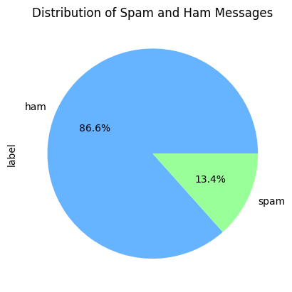
Pie-chart of Distribution of classes

Generating Word-cloud:

As our dataset contains text dataset so that generating word clouds for relevant words in spam and ham messages provides a visual representation of the most common and relevant terms.

Python3

# Generate WordCloud for Spam Messages
spam_text = ' '.join(sms_data[sms_data['label'] == 'spam']['text'])
spam_wordcloud = WordCloud(width=800, height=400, max_words=100, background_color='white', random_state=42).generate(spam_text)

# Generate WordCloud for Ham Messages
ham_text = ' '.join(sms_data[sms_data['label'] == 'ham']['text'])
ham_wordcloud = WordCloud(width=800, height=400, max_words=100, background_color='white', random_state=42).generate(ham_text)

# Plot the WordClouds
plt.figure(figsize=(10, 4))

plt.subplot(1, 2, 1)
plt.imshow(spam_wordcloud, interpolation='bilinear')
plt.title('Word Cloud for Spam Messages')
plt.axis('off')

plt.subplot(1, 2, 2)
plt.imshow(ham_wordcloud, interpolation='bilinear')
plt.title('Word Cloud for Ham Messages')
plt.axis('off')

plt.tight_layout()
plt.show()

Output:

Word cloud for both type of messages

Model Training

Before training models we need to vectorize the text data to convert it to numerical dataset. To do this we will use Count Vectorizer. After that we will train Multinomial NB and also Gaussian NB to show comparative performance. We need to specify some of the Hyperparameters of MNB which are discussed below:

• alpha: It is the Laplace smoothing parameter which is used to avoid zero probabilities in cases where a feature doesn’t occur in a particular class in the training data. A higher value of alpha results in less aggressive smoothing which allows the model to be more sensitive to the training data.
• fit_prior: This is a Boolean parameter (True/False) which determines whether to learn class prior probabilities or not. We will set it to ‘True’ so that it assumes uniform prior probabilities for classes.
• force_alpha: This is also a Boolean parameter (True/False) which forces the alpha to be added to the sample counts and smoothed if it is set to ‘True’.

Python3

# Create a CountVectorizer to convert text data into numerical features
vectorizer = CountVectorizer()
X_train_vec = vectorizer.fit_transform(X_train)
X_test_vec = vectorizer.transform(X_test)

# Train a Multinomial Naive Bayes classifier
mnb = MultinomialNB(alpha=0.8, fit_prior=True, force_alpha=True)
mnb.fit(X_train_vec, y_train)

# Train a Gaussian Naive Bayes classifier
gnb = GaussianNB()
gnb.fit(X_train_vec.toarray(), y_train)

Model Evaluation

Now we will evaluate both the models’ performance in the terms of Accuracy and F1-score.

Python3

# Evaluate the models using accuracy and F1-score
y_pred_mnb = mnb.predict(X_test_vec)
accuracy_mnb = accuracy_score(y_test, y_pred_mnb)
f1_mnb = f1_score(y_test, y_pred_mnb, pos_label='spam')

y_pred_gnb = gnb.predict(X_test_vec.toarray())
accuracy_gnb = accuracy_score(y_test, y_pred_gnb)
f1_gnb = f1_score(y_test, y_pred_gnb, pos_label='spam')

# Print the results
print("Multinomial Naive Bayes - Accuracy:", accuracy_mnb)
print("Multinomial Naive Bayes - F1-score for 'spam' class:", f1_mnb)

print("Gaussian Naive Bayes - Accuracy:", accuracy_gnb)
print("Gaussian Naive Bayes - F1-score for 'spam' class:", f1_gnb)

Output:

Multinomial Naive Bayes - Accuracy: 0.9838565022421525
Multinomial Naive Bayes - F1-score for 'spam' class: 0.9370629370629371
Gaussian Naive Bayes - Accuracy: 0.9004484304932735
Gaussian Naive Bayes - F1-score for 'spam' class: 0.7131782945736436

Comparative visualization

Now we will plot these results to see a comparative visualization of performance for both the models. From the plot we can say that MNB can perform far better than GNB when text data is concerned.

Python3

methods = ['Multinomial Naive Bayes', 'Gaussian Naive Bayes']
accuracy_scores = [accuracy_mnb, accuracy_gnb]
f1_scores = [f1_mnb, f1_gnb]

plt.figure(figsize=(10, 4))
plt.subplot(1, 2, 1)
plt.bar(methods, accuracy_scores, color=['blue', 'green'])
plt.ylabel('Accuracy')
plt.title('Accuracy Comparison')

plt.subplot(1, 2, 2)
plt.bar(methods, f1_scores, color=['blue', 'green'])
plt.ylabel('F1 Score')
plt.title('F1 Score Comparison')

plt.show()

Output:

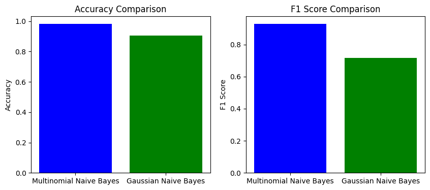
Comparative visualization

Conclusion

We can conclude that MNB is very efficient algorithm for NLP based tasks. Here MNB achieves a notable 98% of accuracy and 93.70% of F1-score which is far better than GNB where F1-score is less.