How to Identify Overfitting Machine Learning Models in Scikit-Learn

Identifying overfitting in machine learning models is crucial to ensuring their performance generalizes well to unseen data. In this article, we’ll explore how to identify overfitting in machine learning models using scikit-learn, a popular machine learning library in Python.

What is Overfitting?

Overfitting is a common problem in machine learning where a model learns the training data too well, capturing noise or random fluctuations that are not present in the underlying true relationship between the features and the target variable. This results in a model that performs well on the training data but generalizes poorly to new, unseen data. In simpler terms, overfitting occurs when a model is too complex relative to the amount and noisiness of the training data.

Causes of Overfitting:

• Model Complexity: Models with too many parameters relative to the size of the training data are prone to overfitting. These models can capture noise in the data rather than the underlying patterns.
• Insufficient Training Data: If the training dataset is too small, the model may not have enough information to learn the underlying patterns, leading to overfitting.
• High Dimensionality: When dealing with high-dimensional data, such as text or images, it’s easy for models to overfit if not properly regularized or if feature selection/reduction techniques are not applied.
• Noise in the Data: If the training data contains a significant amount of noise or irrelevant features, the model may learn to fit the noise rather than the underlying signal.

Identifying Overfitting Machine Learning Models in Scikit-Learn

Identifying overfitting in machine learning models, including those built using Scikit-Learn, is essential to ensure the model generalizes well to unseen data.

Holdout Validation:

• Split the dataset into training and testing sets.
• Train the model on the training set and evaluate its performance on the testing set.
• If the model performs significantly better on the training set than on the testing set, it may be overfitting.

Cross-Validation:

• Perform k-fold cross-validation, where the dataset is divided into k subsets (folds).
• Train the model k times, each time using k-1 folds for training and the remaining fold for validation.
• Compute the average performance across all folds.
• If the average performance on validation sets is significantly worse than on training sets, the model may be overfitting.

Learning Curves:

• Plot the learning curves, showing how model performance (e.g., error or accuracy) changes with training set size.
• If the training error is much lower than the validation error, it suggests overfitting.
• As the training set size increases, the training and validation errors should converge if the model is not overfitting.

Regularization:

• Apply regularization techniques such as L1 or L2 regularization to penalize large model coefficients.
• Tune the regularization hyperparameters using cross-validation to find the optimal balance between model complexity and generalization.

Feature Importance:

• Analyze feature importance scores to identify which features the model relies on most heavily.
• If the model assigns high importance to irrelevant or noisy features, it may be overfitting.

Model Complexity:

• Evaluate the effect of changing the model complexity (e.g., polynomial degree in polynomial regression) on performance.
• If increasing model complexity leads to a significant improvement in training performance but not in testing performance, the model may be overfitting.

Validation Curves:

• Plot validation curves, which show how model performance changes with different hyperparameter values.
• Identify the hyperparameter values that optimize validation performance without overfitting.

Example of how to identify Overfitting Machine Learning Model:

We can identify if a model is overfitted by observing the behavior of the mean squared error (MSE) on the testing set as the polynomial degree increases.

• Decrease in Training Error: As the polynomial degree increases, the model complexity increases, and it becomes more capable of fitting the training data. Consequently, the training error tends to decrease because the model fits the training data more closely.
• Initial Decrease in Testing Error: Initially, with the increase in polynomial degree, the testing error may decrease. This is because the model captures more complexity from the data, resulting in a better fit to the testing data as well.
• Subsequent Increase in Testing Error: After reaching a certain degree of polynomial features, the testing error may start to increase. This increase indicates that the model is becoming too complex and is starting to fit the noise in the training data rather than capturing the underlying pattern. This phenomenon is known as overfitting.

Code Implementation of Identifying Overfitted Model

• Libraries imported: numpy, matplotlib.pyplot, train_test_split, PolynomialFeatures, LinearRegression, mean_squared_error.
• Synthetic data created: x array from 0 to 10, y values computed as sine of x plus noise.
• Data split into training and testing sets: 70% training, 30% testing.
• Models fitted with degrees 1, 3, 10, and 20:
• Polynomial features generated.
• Linear regression models trained.
• Mean squared errors computed for training and testing sets.
• Plot shows relationship between polynomial degree and mean squared error.
• Train error (blue line) and test error (orange line) plotted against polynomial degree.
• Interpretation: Underfitting (low degree), optimal complexity (moderate degree), overfitting (high degree).

Python3

import numpy as np
import matplotlib.pyplot as plt
from sklearn.model_selection import train_test_split
from sklearn.preprocessing import PolynomialFeatures
from sklearn.linear_model import LinearRegression
from sklearn.metrics import mean_squared_error

# Generate synthetic data
np.random.seed(0)
x = np.linspace(0, 10, 100)
y = np.sin(x) + np.random.normal(scale=0.2, size=x.shape)

# Split data into training and testing sets
x_train, x_test, y_train, y_test = train_test_split(x, y, test_size=0.3, random_state=0)

# Fit polynomial regression models of different degrees
degrees = [1, 3, 10, 20]
train_errors = []
test_errors = []

for degree in degrees:
    poly_features = PolynomialFeatures(degree=degree)
    x_poly_train = poly_features.fit_transform(x_train[:, np.newaxis])
    x_poly_test = poly_features.transform(x_test[:, np.newaxis])
    
    model = LinearRegression()
    model.fit(x_poly_train, y_train)
    
    train_predictions = model.predict(x_poly_train)
    test_predictions = model.predict(x_poly_test)
    
    train_errors.append(mean_squared_error(y_train, train_predictions))
    test_errors.append(mean_squared_error(y_test, test_predictions))

# Plot learning curves
plt.figure(figsize=(10, 6))
plt.plot(degrees, train_errors, label='Train Error', marker='o')
plt.plot(degrees, test_errors, label='Test Error', marker='o')
plt.title('Learning Curves')
plt.xlabel('Polynomial Degree')
plt.ylabel('Mean Squared Error')
plt.xticks(degrees)
plt.legend()
plt.grid(True)
plt.show()

Output:

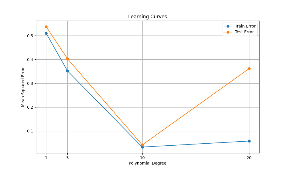
The output of the above code is a plot showing the learning curves for polynomial regression models with different degrees.

• X-axis (Polynomial Degree) represents the degree of the polynomial features used in the regression models. The degrees are chosen from the list [1, 3, 10, 20].
• Y-axis (Mean Squared Error) represents the mean squared error (MSE) of the model’s predictions. Lower values indicate better performance.
• Train Error (Blue Line with Circles): Decreases initially, then remains relatively constant.
• Test Error (Orange Line with Circles): Decreases initially, then increases after a certain degree.

• Underfitting (Low Polynomial Degree): When the polynomial degree is low (e.g., degree 1), the model is too simple to capture the underlying trend in the data, resulting in high errors both on the training and testing sets.
• Optimal Complexity (Moderate Polynomial Degree): There is an optimal degree of the polynomial (around 3 or 10 in this case) where the model achieves the lowest test error, indicating a good balance between bias and variance.
• Overfitting (High Polynomial Degree): When the polynomial degree becomes too high (e.g., degree 20), the model becomes overly complex and starts fitting to noise in the training data. This leads to a decrease in training error but an increase in testing error, indicating poor generalization to new data.

By observing the learning curves, we can identify overfitting by looking for a large gap between the training and testing error. In this example, if the training error is much lower than the testing error, it indicates overfitting.

In the learning curves plot, if you observe a decreasing trend in the testing error followed by an increasing trend after a certain degree of polynomial features, it indicates that the model is overfitted.

Conclusion

In conclusion, identifying overfitting in machine learning models is crucial for ensuring their generalization performance. Here we explored techniques such as holdout validation, cross-validation, learning curves, regularization, and feature importance analysis, all implemented using Scikit-Learn. By carefully evaluating model performance and tuning hyperparameters, practitioners can build more robust models that generalize well to unseen data.