Canonical Correlation Analysis (CCA) using Sklearn

Canonical Correlation Analysis (CCA) is a statistical method used in data analysis to identify and quantify the relationships between two sets of variables. When working with multivariate data—that is, when there are several variables in each of the two sets and we want to know how they connect—it is very helpful. This post will explain CCA, go over its basic terms, and show you how to use the scikit-learn package in Python to implement it (sklearn).

Canonical Correlation Analysis (CCA)

A statistical method for examining and measuring correlations between two sets of variables is called Canonical Correlation Analysis (CCA). Fundamentally, CCA looks for linear combinations of variables—also referred to as canonical variables—within each set so that the correlation between them is maximized. Finding relationships and patterns of linkage between the two groups is the main objective.

Let’s take a practical example where we have two datasets, X and Y, each with many variables. By using canonical variates to describe the linear combinations of variables in X and Y, CCA maximizes the correlation between the canonical variates. The two datasets’ covariation patterns are represented by these canonical variates. These relationships’ strength is measured by the canonical correlations.

When working with high-dimensional datasets where comprehending the intricate correlations between variables is necessary, CCA is especially helpful. Applications in genetics, psychology, economics, and other fields are among its many. For example, CCA in psychology can show correlations between behavioral variables and psychological exams. CCA can detect associated gene expressions in genomics under various experimental setups. CCA helps researchers find significant insights and make wise judgments across a range of fields by offering a thorough perspective of relationships between sets of variables. This enables a deeper understanding of the underlying patterns and linkages in multidimensional data.

Primary Terminologies of Canonical Correlation Analysis (CCA)

Before we dive into the implementation of CCA, let’s define some primary terminologies:

1. Canonical Variables: These are the linear combinations of the original variables in each dataset that maximize the correlation between the two sets. Canonical variables are what CCA aims to find.
2. Canonical Correlations: These are the correlation coefficients between the canonical variables in the two datasets. The goal of CCA is to maximize these correlations.
3. Canonical Loadings: The coefficients known as canonical loadings specify the linear combinations of the original variables that were utilized to produce the canonical variables.
4. Canonical Variates: These are the canonical variables themselves.
5. Cross-Loadings: The association between variables from one dataset and the canonical variables from the other dataset is displayed using cross-loadings.

Mathematical Concept of Canonical Correlation Analysis (CCA)

A statistical technique called canonical correlation analysis (CCA) looks for linear correlations between two sets of data. It is frequently used to examine the connection between various dataset aspects, such as the link between text and pictures or between clinical outcomes and gene expression. A dataset’s dimensionality can also be decreased via CCA by projecting it onto a lower-dimensional subspace while maintaining the correlation structure.

Finding two sets of linear combinations of the original variables—referred to as canonical variables—that have the highest possible degree of correlation with one another is the fundamental notion behind CCA. Assume, for illustration purposes, that we have two sets of variables, X and Y, each having p and q dimensions. To determine which linear combinations of X and have the highest correlation, CCA looks for two vectors, u and v. In terms of math, this may be expressed as:

This is equivalent to solving the following eigenvalue problem:

where lambda is the squared correlation between and , and v is given by:

The solution u and v are called the first pair of canonical variables. They capture the most correlation between X and Y. To find the second pair of canonical variables, we repeat the same process, but with the additional constraint that they are uncorrelated with the first pair. This can be done by removing the projections of X and Y onto the first pair of canonical variables and applying CCA to the residuals. This process can be continued until we obtain min(p, q) pairs of canonical variables, each with decreasing correlation.

Now that we have an understanding of these terminologies, let’s go through the steps of implementing CCA using scikit-learn.

Implementation of Canonical Correlation Analysis (CCA)

To perform CCA in Python, we can use the sklearn.cross_decomposition.CCA class from the scikit-learn library. This class provides methods to fit, transform, and score the CCA model. The fit method takes two arrays, X and Y, as input, and computes the canonical variables. The transform method returns the canonical variables as output, given X and Y. The score method returns the correlation between the canonical variables, given X and Y.

Here is an example of how to use the CCA class:

Using Synthetic Dataset

In this example, we will use a synthetic dataset with two sets of variables, X and Y, each with 10 dimensions. The variables in X and Y are correlated with each other, but not with the variables in the other set. We will use the numpy library to generate the data and apply CCA to find the canonical variables.

Import the libraries

Python

# Import the libraries
import pandas as pd
import numpy as np
from sklearn.cross_decomposition import CCA
import matplotlib.pyplot as plt
import seaborn as sns

• NumPy: for generating and manipulating arrays
• sklearn: for performing CCA
• matplotlib: for plotting the results

Generate the data

Python

# Set the random seed for reproducibility
np.random.seed(0)

# Generate X and Y with 10 dimensions each
X = np.random.randn(100, 10)
Y = X + np.random.randn(100, 10)

To make the code sample reproducible, the random seed is set to 0. Then, two matrices, X and Y, are created, each having 100 rows and 10 columns. The values in matrix X are derived from a typical normal distribution, whilst the values in matrix Y are affected by random noise, adding variability.

Perform CCA

Python

# Create an instance of the CCA class with two components
cca = CCA(n_components=2)

# Fit the CCA model to X and Y
cca.fit(X, Y)

# Transform X and Y to canonical variables
X_c, Y_c = cca.transform(X, Y)

# Score the CCA model
score = cca.score(X, Y)

# Print the score
print(score)

Output:

0.15829448073153862

This snippet of code uses scikit-learn to carry out Canonical Correlation Analysis (CCA). A two-component instance of the CCA class is created, the CCA model is fitted to the matrices X and Y, converting them into canonical variables (X_c and Y_c), and the score—a measure of the correlation between the canonical variables—is computed. The printed score shows how well the CCA model fits the provided data.

Plot the results

We will use the matplotlib. pyplot library to plot the canonical variables. We will create two scatter plots, one for the first pair of canonical variables, and one for the second pair. We will label the axes and add titles to the plots.

Python

# Plot the first pair of canonical variables
plt.scatter(X_c[:, 0], Y_c[:, 0])
plt.xlabel('X_c1')
plt.ylabel('Y_c1')
plt.title('First pair of canonical variables')
plt.show()

# Plot the second pair of canonical variables
plt.scatter(X_c[:, 1], Y_c[:, 1])
plt.xlabel('X_c2')
plt.ylabel('Y_c2')
plt.title('Second pair of canonical variables')
plt.show()

Output:

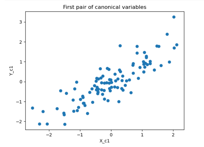
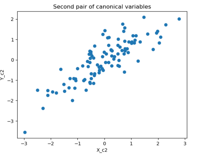
The plots show that the first pair of canonical variables are highly correlated, while the second pair is not. This is consistent with the fact that X and Y are correlated with each other, but not with the variables in the other set.

Using Parkinsons Telemonitoring Data Set

We will utilize the “Parkinsons Telemonitoring Data Set,” a genuine dataset from the UCI Machine Learning Repository, in this example. 42 patients with Parkinson’s disease are featured in 5875 recordings in this dataset, employing a variety of speech signals. Predicting the motor and total UPDRS scores—clinical indicators of the disease’s severity—is the aim. There are two goal variables and 22 characteristics in the dataset.

We will use the pandas library to load the data and split it into X and Y. We will then apply CCA to find the canonical variables and plot the results.

Import the libraries

Python

# Import the libraries
import pandas as pd
import numpy as np
from sklearn.cross_decomposition import CCA
import matplotlib.pyplot as plt

Load and split the data

Python

# Load the data from the URL
data = pd.read_csv('https://archive.ics.uci.edu/ml/machine-learning-databases/parkinsons/telemonitoring/parkinsons_updrs.data')

# Split the data into X and Y
X = data.iloc[:, 6:28]
Y = data.iloc[:, 4:6]

We will use the pandas.read_csv function to load the data from a CSV file. We will then split the data into X and Y, where X contains the 22 features, and Y contains the two target variables.

Perform CCA

Python

# Create an instance of the CCA class with two components
cca = CCA(n_components=2)

# Fit the CCA model to X and Y
cca.fit(X, Y)

# Transform X and Y to canonical variables
X_c, Y_c = cca.transform(X, Y)

# Score the CCA model
score = cca.score(X, Y)

# Print the score
print(score)

Output:

0.007799221129981382

We will use the same CCA class as in the previous example, with two components. We will fit the CCA model to X and Y, and transform them to the canonical variables. We will also score the CCA model, which returns the correlation between the canonical variables. This means that the correlation between the canonical variables is moderate, which indicates a moderate relationship.

Plot the results

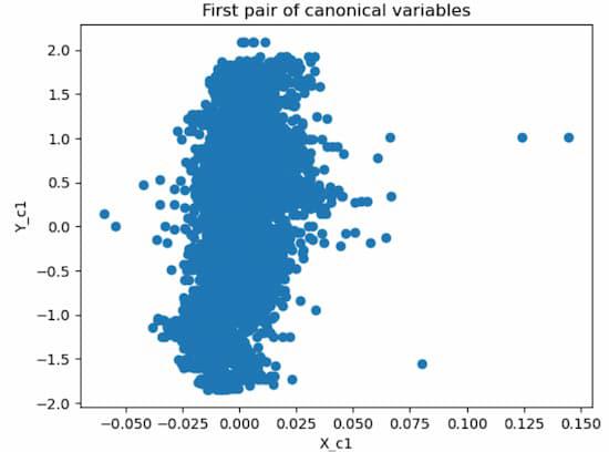
We will use the same matplotlib.pyplot library as in the previous example, to plot the canonical variables. We will create two scatter plots, one for the first pair of canonical variables, and one for the second pair. We will label the axes and add titles to the plots.

Python

# Plot the first pair of canonical variables
plt.scatter(X_c[:, 0], Y_c[:, 0])
plt.xlabel('X_c1')
plt.ylabel('Y_c1')
plt.title('First pair of canonical variables')
plt.show()

# Plot the second pair of canonical variables
plt.scatter(X_c[:, 1], Y_c[:, 1])
plt.xlabel('X_c2')
plt.ylabel('Y_c2')
plt.title('Second pair of canonical variables')
plt.show()

Output:

The plots show that the first pair of canonical variables are moderately correlated, while the second pair is weakly correlated. This suggests that there is some relationship between the speech features and the UPDRS scores, but not very strong.

Plotting Correlation Matrix

Python3

# Calculate the correlation matrix between canonical variables
correlation_matrix = np.corrcoef(X_c.T, Y_c.T)


# Plot the correlation matrix as a heatmap
plt.figure(figsize=(6,4))
sns.heatmap(correlation_matrix, annot=True, cmap='Set2', xticklabels=[
            'X_c1', 'X_c2'], yticklabels=['Y_c1', 'Y_c2'])
plt.title('Canonical Variables Correlation Matrix')
plt.show()

Output:

Correlation Matrix

The correlation matrix between the canonical variables obtained by Canonical Correlation Analysis (CCA) is computed by this code. The canonical variable matrices X_c.T and Y_c.T are transposed when creating the matrix using the np.corrcoef function. Next, using Seaborn’s sns.heatmap, the correlation matrix that results is shown as a heatmap. To improve clarity, the heatmap cells are annotated with numbers using the annot=True option, and the colormap ‘Set2’ is selected for enhanced viewing. The pairwise correlations between the canonical variables are shown by the plot that results when the labels for the x- and y-axes are set appropriately.

Conclusion

In this article, we have explained the concept of canonical correlation analysis, how it works, and how to implement it using the scikit-learn library in Python. Additionally, we have given some instances of using CCA on both fictitious and actual data. CCA is a helpful method for reducing a dataset’s dimensionality and exploring the correlation pattern between two sets of variables. The assumption of linearity, the susceptibility to outliers, and the challenge of interpretation are some of the drawbacks of CCA, though. As a result, it’s critical to exercise caution while using CCA and to confirm the findings using additional techniques.