ML | Variational Bayesian Inference for Gaussian Mixture

Prerequisites: Gaussian Mixture

A Gaussian Mixture Model assumes the data to be segregated into clusters in such a way that each data point in a given cluster follows a particular Multi-variate Gaussian distribution and the Multi-Variate Gaussian distributions of each cluster is independent of one another. To cluster data in such a model, the posterior probability of a data-point belonging to a given cluster given the observed data needs to be calculated. An approximate method for this purpose is the Baye’s method. But for large datasets, the calculation of marginal probabilities is very tedious. As there is only a need to find the most probable cluster for a given point, approximation methods can be used as they reduce the mechanical work. One of the best approximate methods is to use the Variational Bayesian Inference method. The method uses the concepts of KL Divergence and Mean-Field Approximation.

The below steps will demonstrate how to implement Variational Bayesian Inference in a Gaussian Mixture Model using Sklearn. The data used is the Credit Card data which can be downloaded from Kaggle.

Step 1: Importing the required libraries

import numpy as np
import pandas as pd
import matplotlib.pyplot as plt
from sklearn.mixture import BayesianGaussianMixture
from sklearn.preprocessing import normalize, StandardScaler
from sklearn.decomposition import PCA

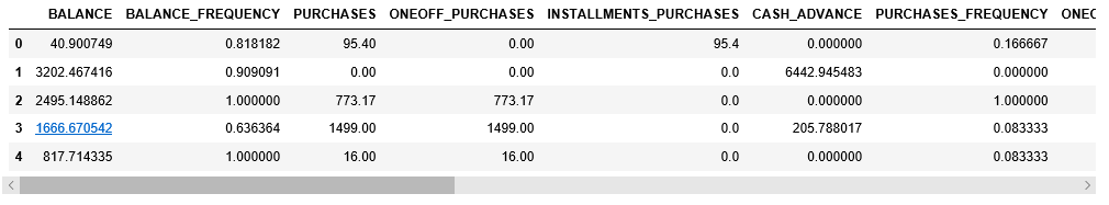
Step 2: Loading and Cleaning the data

# Changing the working location to the location of the data
cd "C:\Users\Dev\Desktop\Kaggle\Credit_Card"

# Loading the Data
X = pd.read_csv('CC_GENERAL.csv')

# Dropping the CUST_ID column from the data
X = X.drop('CUST_ID', axis = 1)

# Handling the missing values
X.fillna(method ='ffill', inplace = True)

X.head()

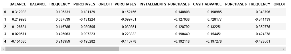
Step 3: Pre-processing the data

# Scaling the data to bring all the attributes to a comparable level
scaler = StandardScaler()
X_scaled = scaler.fit_transform(X)

# Normalizing the data so that the data
# approximately follows a Gaussian distribution
X_normalized = normalize(X_scaled)

# Converting the numpy array into a pandas DataFrame
X_normalized = pd.DataFrame(X_normalized)

# Renaming the columns
X_normalized.columns = X.columns

X_normalized.head()

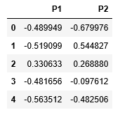
Step 4: Reducing the dimensionality of the data to make it visualizable

# Reducing the dimensions of the data
pca = PCA(n_components = 2)
X_principal = pca.fit_transform(X_normalized)

# Converting the reduced data into a pandas dataframe
X_principal = pd.DataFrame(X_principal)

# Renaming the columns
X_principal.columns = ['P1', 'P2']

X_principal.head()

The primary two parameters of the Bayesian Gaussian Mixture Class aren_components and covariance_type.

1. n_components: It determines the maximum number of clusters in the given data.
2. covariance_type: It describes the type of covariance parameters to be used.

You can read about all the other attributes in it’s documentation.

In the below-given steps, the parameter n_components will be fixed at 5 while the parameter covariance_type will be varied for all possible values to visualize the impact of this parameter on the clustering.

Step 5: Building clustering models for different values of covariance_type and visualizing the results

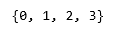
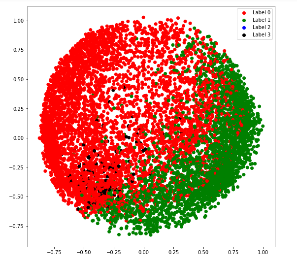
a) covariance_type = ‘full’

# Building and training the model
vbgm_model_full = BayesianGaussianMixture(n_components = 5, covariance_type ='full')
vbgm_model_full.fit(X_normalized)

# Storing the labels
labels_full = vbgm_model_full.predict(X)
print(set(labels_full))

colours = {}
colours[0] = 'r'
colours[1] = 'g'
colours[2] = 'b'
colours[3] = 'k'

# Building the colour vector for each data point
cvec = [colours[label] for label in labels_full]

# Defining the scatter plot for each colour
r = plt.scatter(X_principal['P1'], X_principal['P2'], color ='r');
g = plt.scatter(X_principal['P1'], X_principal['P2'], color ='g');
b = plt.scatter(X_principal['P1'], X_principal['P2'], color ='b');
k = plt.scatter(X_principal['P1'], X_principal['P2'], color ='k');

# Plotting the clustered data
plt.figure(figsize =(9, 9))
plt.scatter(X_principal['P1'], X_principal['P2'], c = cvec)
plt.legend((r, g, b, k), ('Label 0', 'Label 1', 'Label 2', 'Label 3'))
plt.show()

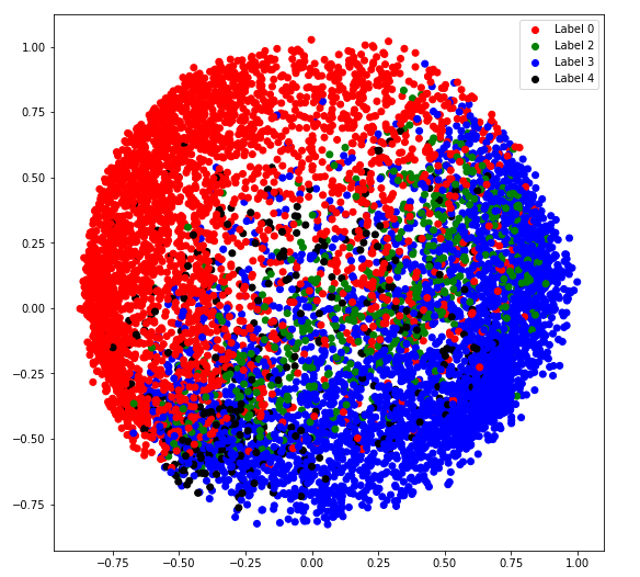
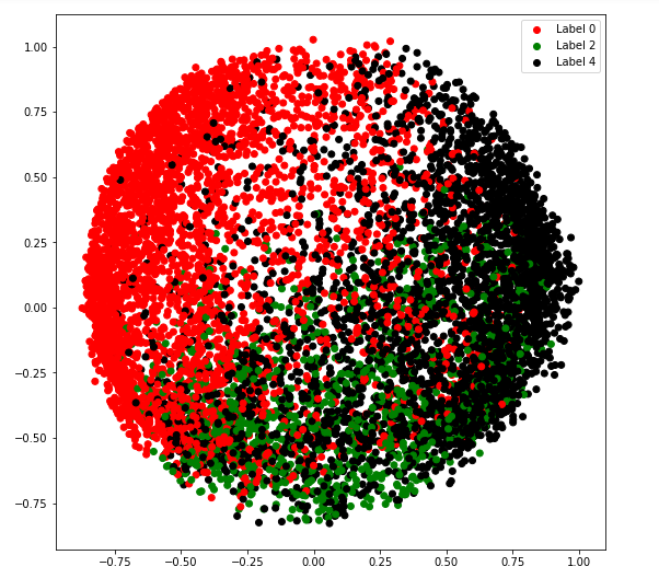
b) covariance_type = ‘tied’

# Building and training the model
vbgm_model_tied = BayesianGaussianMixture(n_components = 5, covariance_type ='tied')
vbgm_model_tied.fit(X_normalized)

# Storing the labels
labels_tied = vbgm_model_tied.predict(X)
print(set(labels_tied))

colours = {}
colours[0] = 'r'
colours[2] = 'g'
colours[3] = 'b'
colours[4] = 'k'

# Building the colour vector for each data point
cvec = [colours[label] for label in labels_tied]

# Defining the scatter plot for each colour
r = plt.scatter(X_principal['P1'], X_principal['P2'], color ='r');
g = plt.scatter(X_principal['P1'], X_principal['P2'], color ='g');
b = plt.scatter(X_principal['P1'], X_principal['P2'], color ='b');
k = plt.scatter(X_principal['P1'], X_principal['P2'], color ='k');

# Plotting the clustered data
plt.figure(figsize =(9, 9))
plt.scatter(X_principal['P1'], X_principal['P2'], c = cvec)
plt.legend((r, g, b, k), ('Label 0', 'Label 2', 'Label 3', 'Label 4'))
plt.show()

c) covariance_type = ‘diag’

# Building and training the model
vbgm_model_diag = BayesianGaussianMixture(n_components = 5, covariance_type ='diag')
vbgm_model_diag.fit(X_normalized)

# Storing the labels
labels_diag = vbgm_model_diag.predict(X)
print(set(labels_diag))

colours = {}
colours[0] = 'r'
colours[2] = 'g'
colours[4] = 'k'

# Building the colour vector for each data point
cvec = [colours[label] for label in labels_diag]

# Defining the scatter plot for each colour
r = plt.scatter(X_principal['P1'], X_principal['P2'], color ='r');
g = plt.scatter(X_principal['P1'], X_principal['P2'], color ='g');
k = plt.scatter(X_principal['P1'], X_principal['P2'], color ='k');

# Plotting the clustered data
plt.figure(figsize =(9, 9))
plt.scatter(X_principal['P1'], X_principal['P2'], c = cvec)
plt.legend((r, g, k), ('Label 0', 'Label 2', 'Label 4'))
plt.show()

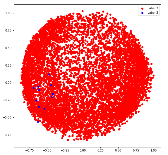
d) covariance_type = ‘spherical’

# Building and training the model
vbgm_model_spherical = BayesianGaussianMixture(n_components = 5,
                                              covariance_type ='spherical')
vbgm_model_spherical.fit(X_normalized)

# Storing the labels
labels_spherical = vbgm_model_spherical.predict(X)
print(set(labels_spherical))

colours = {}
colours[2] = 'r'
colours[3] = 'b'

# Building the colour vector for each data point
cvec = [colours[label] for label in labels_spherical]

# Defining the scatter plot for each colour
r = plt.scatter(X_principal['P1'], X_principal['P2'], color ='r');
b = plt.scatter(X_principal['P1'], X_principal['P2'], color ='b');

# Plotting the clustered data
plt.figure(figsize =(9, 9))
plt.scatter(X_principal['P1'], X_principal['P2'], c = cvec)
plt.legend((r, b), ('Label 2', 'Label 3'))
plt.show()