In this article, we will be making a project through Python language which will be using some Machine Learning Algorithms too. It will be an exciting one as after this project you will understand the concepts of using AI & ML with a scripting language. The following libraries/packages will be used in this project:
- numpy: It’s a Python library that is employed for scientific computing. It contains among other things – a strong array object, mathematical and statistical tools for integrating with other language’s code i.e. C/C++ and Fortran code.
- pandas: It’s a Python package providing fast, flexible, and expressive data structures designed to form working with “relational” or “labeled” data both easy and intuitive.
- matplotlib: Matplotlib may be a plotting library for the Python programming language which produces 2D plots to render visualization and helps in exploring the info sets. matplotlib.pyplot could be a collection of command style functions that make matplotlib work like MATLAB.
- seaborn:. Seaborn is an open-source Python library built on top of matplotlib. It’s used for data visualization and exploratory data analysis. Seaborn works easily with dataframes and also the Pandas library.
Python3
import warnings
warnings.filterwarnings('ignore')
|
After this step we will install some dependencies: Dependencies are all the software components required by your project in order for it to work as intended and avoid runtime errors. We will be needing the numpy, pandas, matplotlib & seaborn libraries / dependencies. As we will need a CSV file to do the operations, for this project we will be using a CSV file that contains data for Tumor (brain disease). So in this project at last we will be able to predict whether a subject (candidate) has a potent chance of suffering from a Tumor or not?
Step 1: Pre-processing the Data:
Python3
import numpy as np
import pandas as pd
import matplotlib.pyplot as plt
import seaborn as sns
|
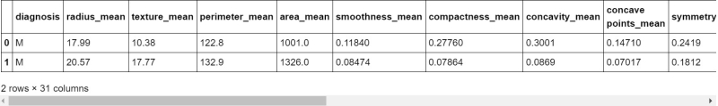
Now we will check that the CSV file has been read successfully or not? So we will use the head method: head() method is used to return top n (5 by default) rows of a data frame or series.
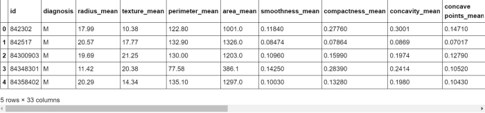
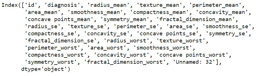
So this command will fetch the column’s header names. The output will be this:
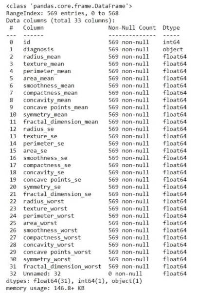
Now in order to understand the data set briefly by getting a quick overview of the data-set, we will use info() method. This method very well handles the exploratory analysis of the data-sets.
Output for above command:
In the CSV file, there may be some blanked fields that can harm the project (that is they will hamper the prediction).
Output:
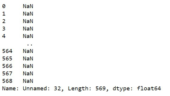
Now as we have successfully found the vacant spaces in the data set, so now we will remove them.
Python3
df = df.drop("Unnamed: 32", axis=1)
df.head()
df.columns
df.drop('id', axis=1, inplace=True)
df.columns
|
Now we will check the class type of the columns with the help of type() method. It returns the class type of the argument(object) passed as a parameter.
Output:
pandas.core.indexes.base.Index
We will be needing to traverse and sort the data by their columns, so we will save the columns in a variable.
Python3
l = list(df.columns)
print(l)
|
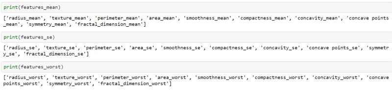
Now we will access the data with different start points. Say we will categorize the columns from 1 to 11 in a variable named features_mean and so on.
Python3
features_mean = l[1:11]
features_se = l[11:21]
features_worst = l[21:]
|
In the ‘Diagnosis’ column of the CSV file, there are two options one is M = Malignant & B = Begin which basically tells the stage of the Tumor. But the same we will verify from the code.
Output:
array(['M', 'B'], dtype=object)
So it verifies that there are only two values in the Diagnosis field.
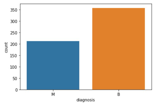
Now in order to get a fair idea of how many cases are having malignant tumor and who are in the beginning stage, we will use the countplot() method.
Python3
sns.countplot(df['diagnosis'], label="Count",);
|
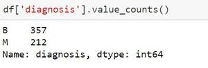
If we don’t have to see the graph for the values, then I can use a function that will return the numerical values of the occurrences.
Now we will be able to be using the shape() method. Shape returns the form of an array. The form could be a tuple of integers. These numbers tell the lengths of the corresponding array dimension. In other words: The “shape” of an array may be a tuple with the number of elements per axis (dimension). For instance, the form is adequate to (6, 3), i.e. we’ve got 6 lines and three columns.
Output:
(539, 31)
which means that in the data set there are 539 lines and 31 columns.
As of now, we are ready with the to-be-processed dataset, so we will be able to be using describe( ) method which is employed to look at some basic statistical details like percentile, mean, std etc. of a knowledge frame or a series of numeric values.
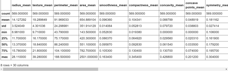
After all, this stuff, we will be using the corr( ) method to find the correlation between different fields. Corr( ) is used to find the pairwise correlation of all columns in the data frame. Any nan values are automatically excluded. For any non-numeric data type columns in the data-frame, it is ignored.
This command will provide 30 rows * 30 columns table which will be having rows like radius_mean, texture_se and so on.
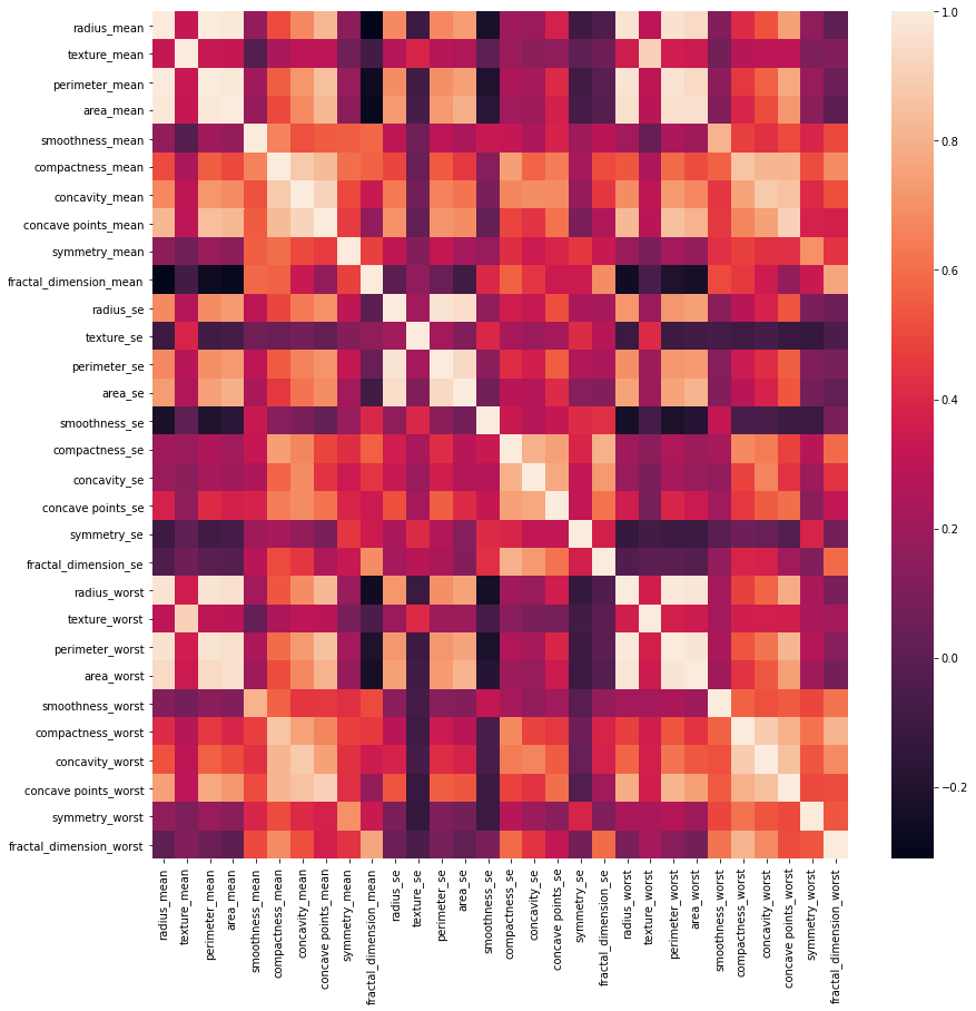
The command corr.shape( ) will return (30, 30). The next step is plotting the statistics via heatmap. A heatmap could even be a two-dimensional graphical representation of information where the individual values that are contained during a matrix are represented as colors. The seaborn package allows the creation of annotated heatmaps which can be changed a little by using Matplotlib tools as per the creator’s requirement.
Python3
plt.figure(figsize=(14, 14))
sns.heatmap(corr)
|
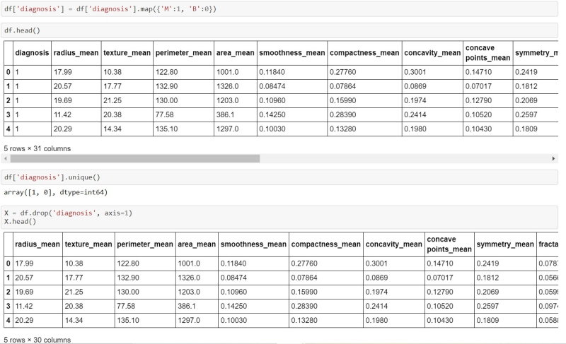
Again we will be checking the CSV data set in order to ensure that the columns are just fine and haven’t been affected by the operations.
This will return a table through which one can be assured that the data set is well sorted or not. In the few next commands, we will be segregating the data.
Python3
df['diagnosis'] = df['diagnosis'].map({'M': 1, 'B': 0})
df.head()
df['diagnosis'].unique()
X = df.drop('diagnosis', axis=1)
X.head()
y = df['diagnosis']
y.head()
|
Note: As we have prepared a prediction model which can be used with any of the machine-learning model, so now we will use one by one show you the output of the prediction model with each of the machine learning algorithms.
Step 2: Test Checking or Training The Data set
- Using Logistic Regression Model:
Python3
from sklearn.preprocessing import StandardScaler
from sklearn.model_selection import train_test_split
X_train, X_test, y_train, y_test = train_test_split(X, y, test_size=0.3)
df.shape
X_train.shape
X_test.shape
y_train.shape
y_test.shape
X_train.head(1)
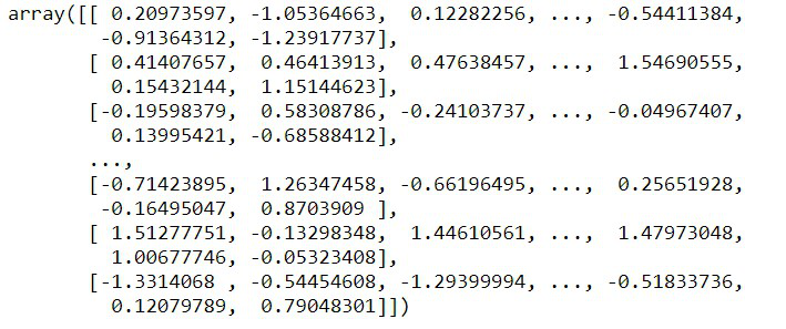
ss = StandardScaler()
X_train = ss.fit_transform(X_train)
X_test = ss.transform(X_test)
X_train
|
Output:
After doing the basic training of the model we can test this by using one of the Machine Learning Models. So we will be testing this by using Logistic Regression, Decision Tree Classifier, Random Forest Classifier and SVM.
Python3
from sklearn.linear_model import LogisticRegression
lr = LogisticRegression()
lr.fit(X_train, y_train)
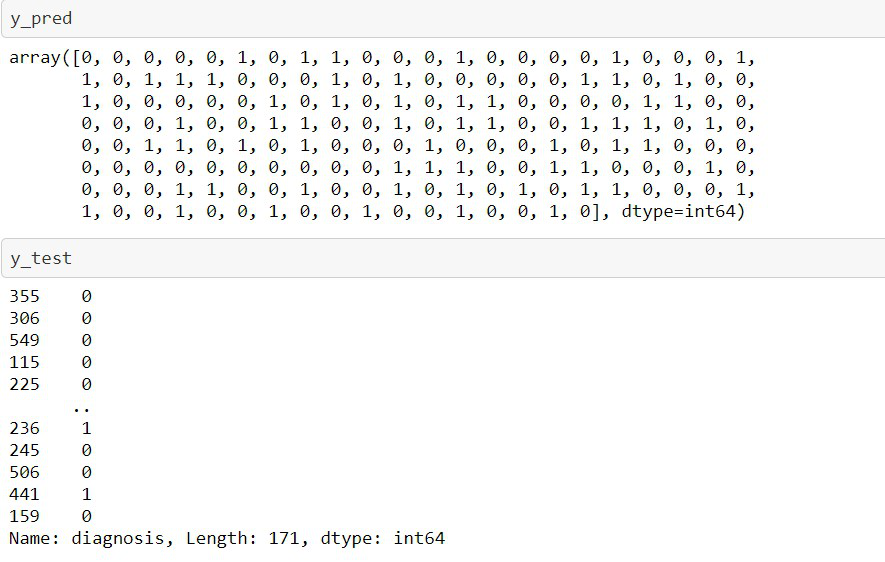
y_pred = lr.predict(X_test)
y_pred
y_test
|
Output:
To mathematically check to what extent the model has predicted the correct value:
Python3
from sklearn.metrics import accuracy_score
print(accuracy_score(y_test, y_pred))
|
Output:
0.9883040935672515
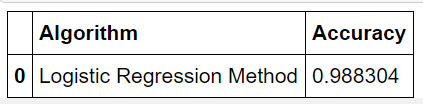
Now let’s frame the results in the form of a table.
Python3
tempResults = pd.DataFrame({'Algorithm':['Logistic Regression Method'], 'Accuracy':[lr_acc]})
results = pd.concat( [results, tempResults] )
results = results[['Algorithm','Accuracy']]
results
|
Output:
- Using Decision Tree Model:
Python3
from sklearn.metrics import accuracy_score
from sklearn.tree import DecisionTreeClassifier
dtc = DecisionTreeClassifier()
dtc.fit(X_train, y_train)
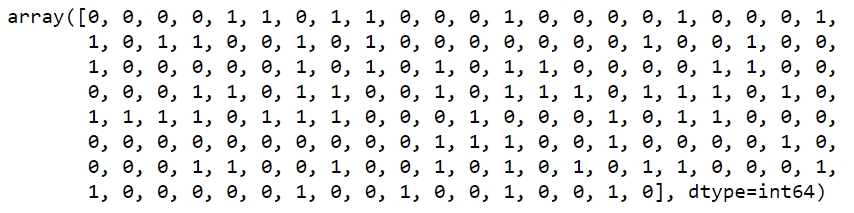
y_pred = dtc.predict(X_test)
y_pred
print(accuracy_score(y_test, y_pred))
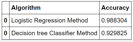
tempResults = pd.DataFrame({'Algorithm': ['Decision tree Classifier Method'],
'Accuracy': [dtc_acc]})
results = pd.concat([results, tempResults])
results = results[['Algorithm', 'Accuracy']]
results
|
Output:
- Using Random Forest Model:
Python3
from sklearn.metrics import accuracy_score
from sklearn.ensemble import RandomForestClassifier
rfc = RandomForestClassifier()
rfc.fit(X_train, y_train)
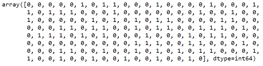
y_pred = rfc.predict(X_test)
y_pred
print(accuracy_score(y_test, y_pred))
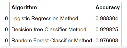
tempResults = pd.DataFrame({'Algorithm': ['Random Forest Classifier Method'],
'Accuracy': [rfc_acc]})
results = pd.concat([results, tempResults])
results = results[['Algorithm', 'Accuracy']]
results
|
Output:
Python3
from sklearn import svm
svc = svm.SVC()
svc.fit(X_train,y_train
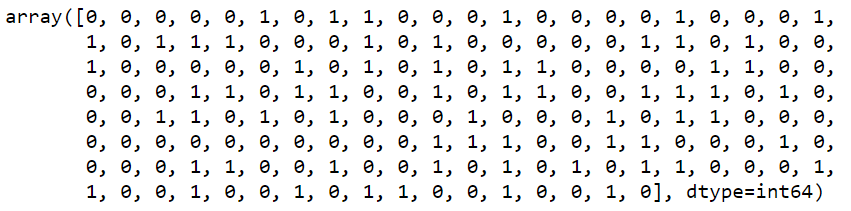
y_pred = svc.predict(X_test)
y_pred
from sklearn.metrics import accuracy_score
print(accuracy_score(y_test, y_pred))
|
Output:
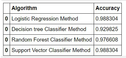
So now we can check that which model effectively produced a higher number of correct predictions through this table:
Python3
tempResults = pd.DataFrame({'Algorithm': ['Support Vector Classifier Method'],
'Accuracy': [svc_acc]})
results = pd.concat([results, tempResults])
results = results[['Algorithm', 'Accuracy']]
results
|
Output:
After going through the accuracy of the above-used machine learning algorithms, I can conclude that these algorithms will give the same output every time if the same data set is fed. I can also say that these algorithms majorly provide the same output of prediction accuracy even if the data set is changed.
From the above table, we can conclude that through SVM Model and Logistic Regression Model were the best-suited models for my project.
Share your thoughts in the comments
Please Login to comment...