The Difference Between rnorm() and runif() in R

While conducting statistical analysis we generate random numbers for reproducibility and experiments. R Programming Language provides two functions runif() and rnorm() to generate random functions. In this article, we will understand the difference between these two functions and how we can use them with the help of examples.

Difference between rnorm() and runif()

We can understand the difference between the rnorm() and runif() functions in tabulated form as well.

Aspect	rnorm()	runif()
Distribution Type	Normal	Uniform
Parameters	n, mean, sd	n, min, max
Shape of Distribution	Bell-shaped, symmetrical around the mean	Flat, constant within the specified range
Example	rnorm(100, mean = 0, sd = 1)	runif(100, min = 0, max = 1)

rnorm()

rnorm() is a popular function in R that generates random numbers using normal distribution. Normal distribution, also called Gaussian distribution, represents a bell-shaped curve with the maximum values clustered around the mean value.
The Probability Density function of a normal distribution is given by:

f(x| μ, σ² ) = 1/√2πσ² e^{-(x-μ)2 / 2σ2}

where,

• x is a random variable
• μ is the mean value
• σ² is the standard deviation

rnorm() function takes three parameters. The standard parameter for this function is given by:

R

rnorm(n, mean = 0, sd = 1)

where,

• n= number of random numbers to be generated
• mean: The mean of the normal distribution. Default is 0.
• sd: The standard deviation of the normal distribution. Default is 1.

The mean parameter decides the center of the distribution while the sd parameter defines the spread of the distribution. We can understand this with the help of a random example and also plot it to understand how this distribution works.

R

# Generate 100 random numbers from a normal distribution with mean 0 and sd 1
random_numbers <- rnorm(100, mean = 0, sd = 1)

# Plot a histogram of the random numbers
hist(random_numbers, freq = FALSE, col = "skyblue",
     main = "Histogram of Random Numbers from Normal Distribution",
     xlab = "Random Numbers", ylab = "Density")

# Add a density curve to the histogram
lines(density(random_numbers), col = "red", lwd = 2)

Output:

Difference Between rnorm() and runif() in R

The above curve is bell-shaped since it is a normal distribution.

Analysis of Height in Adults using rnorm()

Suppose we want to analyze the height of the individuals in a particular country and we need to generate a dataset that closely resembles the actual height of the people in that country. For this purpose, we can use the rnorm() function to analyze the height, average height, standard deviation of height, and the category where most of the heights will fall.

R

# Define parameters based on real-world data or estimates
mean_height <- 170  # Mean height in centimeters
sd_height <- 10     # Standard deviation of heights

# Generate a dataset of 1000 random heights
height_data <- rnorm(1000, mean = mean_height, sd = sd_height)

# Analyze the generated data
mean_height_generated <- mean(height_data)
median_height_generated <- median(height_data)

#to view the first 6 rows of the dataset
head(height_data)

Output:

[1] 166.6658 171.7388 156.5240 170.6069 170.0746 175.0088

Visualize the distribution of heights

R

# Visualize the distribution of heights
hist(height_data, breaks = 20, col = "skyblue", main = "Distribution of Heights",
     xlab = "Height (cm)", ylab = "Frequency")

# Add mean and median lines to the histogram
abline(v = mean_height_generated, col = "red", lwd = 2, lty = 2)

abline(v = median_height_generated, col = "blue", lwd = 2, lty = 2)

# Add legend
legend("topright", legend = c("Mean", "Median"),
       col = c("red", "blue"), lty = 2, lwd = 2)

Output:

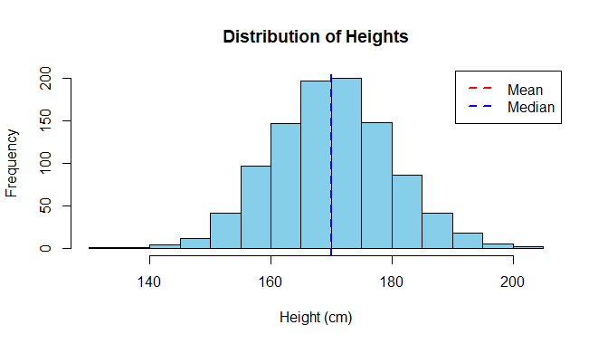
Difference Between rnorm() and runif() in R

This dataset closely resembles real-world observations and allows us to perform various statistical analyses and visualizations, providing insights into the distribution of heights and the characteristics of the population.

runif()

runif() function in R programming language uses uniform distribution to generate random functions. Under this distribution, all the observations are equally likely to occur and it is characterized by a constant probability density function within the range. Uniform Distribution does not have any peak like normal distribution. The values in uniform distribution have equal chances of occurring. It is defined as:

f(x | a, b) = 1/b-a for a ≤ x ≤ b

where,

• x is a random variable
• a is the minimum value
• b is the maximum value

The standard syntax for this function is given by

R

runif(n, min = 0, max = 1)

where,

• n: numbers to be generated randomly
• min: The minimum value of the uniform distribution. Default is 0.
• max: The maximum value of the uniform distribution. Default is 1.

The min and max values generate the range of the distribution and each value within this range has equal probability of getting selected. We can understand this with the help of a random example and also plot it to understand how this distribution works

R

# Generate 100 random numbers from a uniform distribution between 0 and 10
random_numbers <- runif(100, min = 0, max = 10)

# Plot a histogram
hist(random_numbers, breaks = 10, col = "skyblue", main = "Histogram of Random Numbers",
     xlab = "Random Numbers", ylab = "Frequency")

Output:

Difference Between rnorm() and runif() in R

Temperature analysis using runif()

Let us assume we want to perform analysis of temperature of a city recorded over a week. This can help us in planning the outdoor activities or parties, etc.

R

# Set seed for reproducibility
set.seed(123)

# Generate random temperatures for each day of the week (in Celsius)
temperatures <- runif(7, min = 10, max = 30)

#display the data
head(temperatures)

# Define days as a factor to ensure valid finite range
days <- factor(c("Monday", "Tuesday", "Wednesday", "Thursday", "Friday", "Saturday",
                 "Sunday"))

# Create a color palette for gradient colors
colors <- colorRampPalette(c("lightblue", "darkblue"))(length(temperatures))

# Plot graph
barplot(temperatures, names.arg = days, col = colors,
        main = "Temperatures Over the Week",
        xlab = "Day", ylab = "Temperature (°C)", border = "white")

Output:

[1] 15.75155 25.76610 18.17954 27.66035 28.80935 10.91113

Difference Between rnorm() and runif() in R

This approach allows us to understand the variability in temperatures throughout the week and can be useful for making informed decisions related to outdoor activities or climate analysis.

Conclusion

In this article, we understood the difference between the rnorm() and runif() functions with the help of different examples and also visualized them to understand better.