Stock Data Analysis and Data Visualization with Quantmod in R

Analysis of historical stock price and volume data is done in order to obtain knowledge, make wise decisions, and create trading or investment strategies. The following elements are frequently included in the examination of stock data in the R Programming Language.

1. Historical Price Data: Historical price data contains information about a stock’s open, high, low, and closing prices over a specific period, usually daily or intraday.
2. Volume Data: Volume data represents the number of shares traded for a particular stock on a given day. It helps assess the liquidity and interest in the stock.
3. Returns: Returns measure the percentage change in stock prices over time and are used to calculate investment performance.
4. Technical Indicators: Technical indicators, such as moving averages, relative strength index (RSI), and moving average convergence divergence (MACD), are mathematical calculations applied to stock prices and volumes to identify trends and potential buy or sell signals.
5. Statistical Models: Advanced stock analysis may involve statistical models like autoregressive integrated moving averages (ARIMA) or GARCH models for price forecasting and risk assessment.

Stock data analysis using R involves examining the historical price and volume data of a particular stock or financial instrument to make informed investment decisions. Several technical indicators and terms are commonly used in stock data analysis to assess trends, momentum, and potential trading opportunities. Two popular indicators are the Relative Strength Index (RSI) and Moving Average Convergence Divergence (MACD).

Relative Strength Index (RSI)

RSI is a momentum oscillator that measures the speed and change of price movements. It is used to identify overbought or oversold conditions in a stock, which can help traders determine potential reversal points.

Calculation: RSI is typically calculated using the following formula:

RSI = 100 - (100 / (1 + RS))

Where RS (Relative Strength) = Average gain over a specified period / Average loss over the same period.

Interpretation: RSI values range from 0 to 100. Generally, an RSI above 70 indicates that a stock may be overbought and due for a potential pullback, while an RSI below 30 suggests that it may be oversold and due for a potential bounce.

Moving Average Convergence Divergence (MACD):

MACD is a trend-following momentum indicator that shows the relationship between two moving averages of a stock’s price. It helps traders identify changes in the strength, direction, momentum, and duration of a stock’s trend.

MACD is calculated using two exponential moving averages (EMA) and a signal line (a 9-period EMA of the MACD). The formula for MACD is as follows:

MACD Line = 12-period EMA - 26-period EMA
Signal Line = 9-period EMA of MACD Line
MACD Histogram = MACD Line - Signal Line

Quantmod Package:

Quantmod is an R package specifically designed for quantitative financial modeling and trading. It provides a wide range of functions and tools for collecting, analyzing, and visualizing financial and stock market data.
Key features of the Quantmod package include.

Fetching Data: Quantmod allows users to retrieve historical stock data from various sources, including Yahoo Finance and Alpha Vantage, using functions like getSymbols().

1. Installing and Loading the Necessary Packages
2. Load the Apple Stock dataset
3. Data Preprocessing
4. Visualization
5. Modeling

Installing and Loading the Necessary Packages

R

# Install and load the necessary packages
install.packages("quantmod")
library(quantmod)

install.packages("ggplot2")
library(ggplot2)

Load the Apple Stock dataset

R

# Fetch historical stock data for Apple Inc. (AAPL) from Yahoo Finance
getSymbols("AAPL", from = "2020-01-01", to = "2021-12-31")

# View the first few rows of the data
head(AAPL)

Output:

           AAPL.Open AAPL.High AAPL.Low AAPL.Close AAPL.Volume AAPL.Adjusted
2020-01-02   74.0600   75.1500  73.7975    75.0875   135480400      73.24903
2020-01-03   74.2875   75.1450  74.1250    74.3575   146322800      72.53689
2020-01-06   73.4475   74.9900  73.1875    74.9500   118387200      73.11489
2020-01-07   74.9600   75.2250  74.3700    74.5975   108872000      72.77103
2020-01-08   74.2900   76.1100  74.2900    75.7975   132079200      73.94164
2020-01-09   76.8100   77.6075  76.5500    77.4075   170108400      75.51224

getSymbols(“AAPL”, from = “2020-01-01”, to = “2021-12-31”): This line of code fetches historical stock data for AAPL from Yahoo Finance. It specifies the stock symbol (“AAPL”) and the date range (“2020-01-01” to “2021-12-31”) for which you want to retrieve the data. The data will be stored in the variable AAPL.

Data Preprocessing

R

# Clean the data by removing missing values
AAPL_clean <- na.omit(AAPL)

# Calculate daily returns
AAPL_clean$Returns <- dailyReturn(AAPL_clean$AAPL.Adjusted)

# Remove outliers using z-score (assuming you have 'zoo' package installed)
library(zoo)
z_scores <- scale(AAPL_clean$Returns)
AAPL_clean <- AAPL_clean[abs(z_scores) < 3, ]

# Check summary statistics of the cleaned data
summary(AAPL_clean$Returns)

Output:

     Index               Returns         
 Min.   :2020-01-02   Min.   :-0.067295  
 1st Qu.:2020-07-09   1st Qu.:-0.008163  
 Median :2021-01-07   Median : 0.001474  
 Mean   :2021-01-05   Mean   : 0.001821  
 3rd Qu.:2021-07-06   3rd Qu.: 0.013851  
 Max.   :2021-12-30   Max.   : 0.072022 

Basic Stock Data Analysis

R

# Calculate 50-day and 200-day moving averages
AAPL_clean$MA_50 <- SMA(AAPL_clean$AAPL.Adjusted, n = 50)
AAPL_clean$MA_200 <- SMA(AAPL_clean$AAPL.Adjusted, n = 200)

# Calculate historical volatility
AAPL_clean$Volatility <- runSD(AAPL_clean$Returns, n = 20) * sqrt(252)

# Visualize stock data with moving averages and volatility
ggplot(data = AAPL_clean, aes(x = Index)) +
  geom_line(aes(y = AAPL.Adjusted), color = "blue", size = 1) +
  geom_line(aes(y = MA_50), color = "orange", size = 1) +
  geom_line(aes(y = MA_200), color = "red", size = 1) +
  labs(title = "Apple Inc. Stock Price with Moving Averages",
       x = "Date", y = "Price") +
  theme_minimal()

Output:

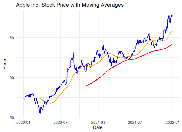
Stock Price with Moving Averages

• AAPL_clean$MA_50 <- SMA(AAPL_clean$AAPL.Adjusted, n = 50): This line of code calculates the 50-day simple moving average (SMA) for AAPL’s adjusted closing prices. It adds a new column named MA_50 to the AAPL_clean data frame to store the moving average values.

• AAPL_clean$MA_200 <- SMA(AAPL_clean$AAPL.Adjusted, n = 200): Similar to the previous line, this code calculates the 200-day simple moving average and stores it in a new column named MA_200.
• AAPL_clean$Volatility <- runSD(AAPL_clean$Returns, n = 20) * sqrt(252): This line calculates the historical volatility. It uses the standard deviation of daily returns over a 20-day period and annualizes it by multiplying by the square root of 252 (the number of trading days in a year). The result is stored in a new column named Volatility.
• ggplot(data = AAPL_clean, aes(x = Index)) + …: This part of the code creates a ggplot2 visualization of the stock data. It uses geom_line() to plot the AAPL adjusted closing prices (in blue), the 50-day moving average (in orange), and the 200-day moving average (in red) against the date (x-axis) and price (y-axis). It sets the title, x-axis label, and y-axis label using the labs() function and applies a minimal theme with theme_minimal().

Plot the closing price of AAPL

R

# Plot the closing price of AAPL
chartSeries(AAPL$AAPL.Close, type = "line", name = "AAPL Closing Price")

Output:

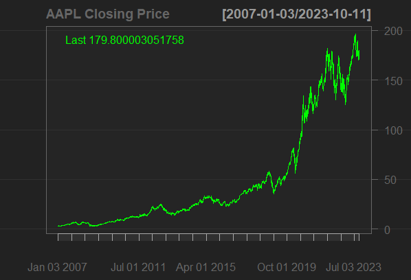
closing price of AAPL with Quantmod

chartSeries: This is the main function that generates the chart. It is used to create various types of financial charts, including line charts, candlestick charts, and more.

• AAPL$AAPL.Close: This part of the code specifies the data you want to plot, which is the closing price of AAPL. In the quantmod package, the data for the stock’s closing price is typically stored in a data frame as AAPL$AAPL.Close.
• type = “line”: This argument specifies that you want to create a line chart. You can change the “line” to other chart types like “candlesticks” or “bars” if you prefer a different visualization style.
• name = “AAPL Closing Price”: This argument is used to set the name or title of the chart. In this case, it labels the chart as “AAPL Closing Price.”

Plot the moving averages

R

# Calculate 20-day, 50-day and 200-day moving averages
AAPL$SMA_20 <- SMA(AAPL$AAPL.Close, n = 20)
AAPL$SMA_50 <- SMA(AAPL$AAPL.Close, n = 50)
AAPL$SMA_100 <- SMA(AAPL$AAPL.Close, n = 100)

# Plot the moving averages
chart_Series(AAPL, name = "AAPL Moving Averages")
add_TA(AAPL$SMA_20, on = 1, col = "blue", lty = 1)
add_TA(AAPL$SMA_50, on = 1, col = "red", lty = 1)
add_TA(AAPL$SMA_100, on = 1, col = "green", lty = 1)

Output:

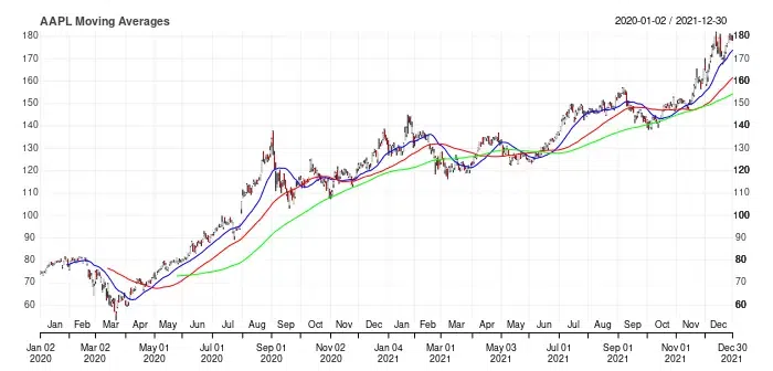
Time Series Moving Averages

• AAPL$SMA_20 <- SMA(AAPL$AAPL.Close, n = 20): This line calculates the 20-day simple moving average (SMA) for the closing price of AAPL. It stores the calculated SMA values in a new column named “SMA_20” in the AAPL data frame.
• AAPL$SMA_50 <- SMA(AAPL$AAPL.Close, n = 50): This line calculates the 50-day simple moving average (SMA) for the closing price of AAPL. It stores the calculated SMA values in a new column named “SMA_50” in the AAPL data frame.
• AAPL$SMA_100 <- SMA(AAPL$AAPL.Close, n = 100): Similarly, this line calculates the 100-day SMA for the closing price and stores the values in a new column named “SMA_100.”
• chart_Series(AAPL, name = “AAPL Moving Averages”): This line creates a chart series for the AAPL data, labeling it as “AAPL Moving Averages.”
• add_TA(AAPL$SMA_20, on = 1, col = “blue”, lty = 1): This line adds the 20-day SMA to the chart. The on argument specifies the subplot to which the indicator should be added (in this case, the main chart), and it is colored blue with a solid line style.
• add_TA(AAPL$SMA_50, on = 1, col = “red”, lty = 1): This line adds the 50-day SMA to the chart. It is also added to the main chart and is colored red with a solid line style.
• add_TA(AAPL$SMA_100, on = 1, col = “green”, lty = 1): This line adds the 100-day SMA to the chart. It is also added to the main chart and is colored red with a solid line style.

Conclusion

In conclusion, a key component of making wise investing choices in the financial markets is stock data analysis. Trading and investing professionals can evaluate trends, momentum, and probable entry or exit points for stocks and other financial instruments by comprehending and using a variety of technical indicators, such as the Moving Average Convergence Divergence (MACD) and Relative Strength Index (RSI).