Similarity Search for Time-Series Data

Time-series analysis is a statistical approach for analyzing data that has been structured through time. It entails analyzing past data to detect patterns, trends, and anomalies, then applying this knowledge to forecast future trends. Time-series analysis has several uses, including in finance, economics, engineering, and the healthcare industry.

Time-series datasets are collections of data points that are recorded over time, such as stock prices, weather patterns, or sensor readings. In many real-world applications, it is often necessary to compare multiple time-series datasets to find similarities or differences between them.

Similarity search, which includes determining the degree to which similarities exist between two or more time-series data sets, is a fundamental task in time-series analysis. This is an essential phase in a variety of applications, including anomaly detection, clustering, and forecasting. In anomaly detection, for example, we may wish to find data points that differ considerably from the predicted trend. In clustering, we could wish to combine time-series data sets that have similar patterns, but in forecasting, we might want to discover the most comparable past data to reliably anticipate future trends.

In time-series analysis, there are numerous approaches for searching for similarities, including the Euclidean distance, dynamic time warping (DTW), and shape-based methods like the Fourier transform and Symbolic Aggregate ApproXimation (SAX). The approach chosen is determined by the individual purpose, the scope and complexity of the data collection, and the amount of noise and outliers in the data.

Although time-series analysis and similarity search are strong tools, they are not without their drawbacks. Handling missing data, dealing with big and complicated data sets, and selecting appropriate similarity metrics, can be challenging. Yet, these obstacles may be addressed with thorough data preparation and the selection of relevant procedures.

Types of similarity measures

Time-series analysis is the process of reviewing previous data to detect patterns, trends, and anomalies and then utilizing this knowledge to forecast future trends. Similarity search, which includes determining the degree to which similarities exist among two or more time-series data sets, is an essential problem in time-series analysis. 

Similarity metrics, which quantify the degree to which there is similarity or dissimilarity among two time-series data sets, are critical in this endeavor. This article will go through the several types of similarity metrics that are often employed in time-series analysis.

Euclidean Distance

Euclidean distance is a distance metric that is widely used to calculate the similarity of two data points in an n-dimensional space. The Euclidean distance is used in time-series analysis to determine the degree of similarity between two time-series data sets with the same amount of observations. This distance metric is sensitive to noise and outliers, and it may not be effective in capturing shape-based similarities. The Euclidean distance between two places A(x1, y1) and B(x2, y2) is calculated as the square root of the sum of the squared differences between the corresponding dimensions of the two data points. 

The Euclidean distance between two time-series data sets with the same number of observations is determined in the context of time-series analysis. The distance between the respective data points is determined at each time point, and the distances are then added together over time to give the overall distance between the two time-series data sets.

In Python, here’s an example of computing Euclidean distance between two time-series data sets:

Python3

# Code for calculating the Euclidean Distance
# between two time-seires data sets.
import numpy as np
# Now let's define two time-series data sets
time_series_A = np.array([1, 2, 3])
time_series_B = np.array([4, 5, 6])
# Now calculating the Euclidean distance using the formula
euclidean_distance = np.sqrt(np.sum(
  (time_series_A - time_series_B)**2))
# Now printing the Euclidean distance
print("Euclidean distance between two time-series is:",
      euclidean_distance)

Output:

Euclidean distance between two time-series is: 5.196152422706632

The advantages of Euclidean distance are as follows:

• Straightforward and quick to compute; 
• works well when time series have comparable shapes and magnitudes.

The Limitations of Euclidean distance are as follows:

• Vulnerable to scaling, 
• outliers, and noise; 
• incompatible with time series of varying forms.

Dynamic Time Warping (DTW)

Dynamic Time Warping (DTW) is a prominent similarity metric in time-series analysis, particularly when the data sets are of varying durations or exhibit phase changes or time warping. DTW, unlike Euclidean distance, allows for non-linear warping of the time axis to suit analogous patterns in time-series data sets. DTW is commonly used in speech recognition, signal processing, and finance.

DTW is a technique for discovering the optimum alignment between two time-series data sets by estimating the cumulative distance between each pair of related data points and calculating the shortest distance path through the cumulative distance matrix. The generated least distance path represents the optimal alignment.

The mathematical representation for Dynamic Time Warping (DTW) can be interpreted as follows: 

Let call ‘time_series_A’ and ‘time_series_B’ be two-time series data sets with lengths of  ‘n’ and ‘m’, respectively. The DTW distance between the first ‘i’th elements of ‘time_series_A’ and the first ‘j’th elements of ‘time-series_B’ denoted by ‘dtw_matrix [i,j]’. 

Let us now apply the following recurrence relation:

D[0,0] = 0
D[i,j] = cost(i,j) + min(D[i-1,j], D[i,j-1], D[i-1,j-1])

where ‘cost(i,j)’ is the cost of aligning the ‘i’th element of ‘time_series_A’ with the ‘j’th element of ‘time_series_B’, and may be computed as the absolute difference between the two values, i.e., ‘cost(i,j) = abs(time_series_A[i-1] – time_series_B[j-1])’. 

In Python, here’s an example of computing Dynamic Time Warping (DTW) distance between two time-series data sets:

Python3

import numpy as np

# Let us now define two time-series data sets
time_series_A = np.array([7, 8, 9, 15])
time_series_B = np.array([4, 6, 7, 3])

# Computing the DTW distance between the two time-series data sets
def dtw_distance(time_series_A, time_series_B):
    n = len(time_series_A)
    m = len(time_series_B)
    dtw_matrix = np.zeros((n+1, m+1))
    for i in range(1, n+1):
        for j in range(1, m+1):
            # Computing the cost by using the above mathematical formula &
            # Finding the absolute difference between two values
            cost = abs(time_series_A[i-1] - time_series_B[j-1])
            dtw_matrix[i, j] = cost + min(dtw_matrix[i-1, j],
                                          dtw_matrix[i, j-1],
                                          dtw_matrix[i-1, j-1])
    return dtw_matrix[n, m]

dtw_distance = dtw_distance(time_series_A, time_series_B)
print("Dynamic Time Warping (DTW) distance :",dtw_distance)

Output:

Dynamic Time Warping (DTW) distance : 15.0

The Dynamic Time Warping (DTW) distance is estimated using a dynamic programming technique, where a cost matrix is built to keep track of the accumulated costs of all potential pathways. The option with the lowest cost is chosen, and the total cost along that path equals the Dynamic Time Warping (DTW) distance between the two time-series data sets.

The advantages of Dynamic Time Warping (DTW) are as follows:

• Resistant to time series scaling, shifting, and warping; 
• can handle time series of varying forms; 
• commonly used in voice and gesture detection.

The limitations of Dynamic Time Warping (DTW) are as follows:

• For lengthy time series, 
• it is computationally costly; 
• it is susceptible to noise and outliers.

Shape-based Methods

Shape-based approaches are a type of similarity measure in which time-series data sets are transformed into a new representation, such as the Fourier transform or Symbolic Aggregate Approximation (SAX), and then compared based on their shape. These approaches are good at collecting shape-based similarities and are commonly used in pattern recognition, clustering, and anomaly identification. Nevertheless, the success of shape-based approaches is dependent on the transformation used and the amount of noise and outliers in the data.

The mathematical equation for the popular shape-based time-series data analysis methodology Symbolic Aggregate Approximation (SAX):

The SAX method turns a time-series data collection ‘ts’ of length ‘n’ and a number of segments ‘m’ into a symbolic representation by splitting it into ‘m’ segments of equal length ‘w = n/m’ and transforming each segment into a symbol based on its mean value. This may be stated as follows:

1. Using a basic normal distribution lookup table, calculate the breakpoints for the required number of symbols (generally represented by ‘a’). The breakpoints are the values that divide the normal distribution into a set of equiprobable zones, and they are represented by the ‘a-1′ quantiles ‘q1, q2,…, q (a-1)’.

2. Compute the mean values of each ‘w-length’ segment in ‘ts’, designated by ‘v1, v2,…, vm’.

3. Based on its position relative to the breakpoints, convert each segment mean value ‘v_i’ to a symbol. Let ‘alpha’ be an ‘m-length’ string made up of the symbols corresponding to each segment mean value, such that:

alpha[i] = j  if  q(j-1) <= v_i < q(j)    (for 1 <= i <= m)

where ‘j’ is an integer between ‘1’ and ‘a’.

4. The string ‘alpha’ is the resultant symbolic representation of ‘ts’.

It is worth noting that the distance is determined by comparing the SAX representations of the two time-series data sets symbol by symbol and adding the squared differences between the relevant breakpoints.

The advantages of Shape-based methods are as follows:

• Converting time-series data sets into a new representation, such as Fourier transform or Symbolic Aggregate approXimation (SAX), then comparing them depending on their shape; 
• can handle time series with diverse forms and magnitudes.

The limitations of Shape-based methods are as follows:

• The transformation used may influence the similarity measure;
• The success of the strategy may be dependent on the specific application.

In Python, here’s an example of computing the Symbolic Aggregate approXimation (SAX) distance time-series data:

Python3

import numpy as np
from sklearn.preprocessing import StandardScaler

def to_sax(time_series, window_size, alphabet_size):
    # Normalize the time series data to have a mean of 0 and a standard deviation of 1.
    scaler = StandardScaler()
    normalized_ts = scaler.fit_transform(time_series.reshape(-1, 1)).flatten()

    # Define the breakpoints for the bins.
    breakpoints = np.linspace(-np.sqrt(2), np.sqrt(2), alphabet_size - 1)

    # Divide the normalized time series into equal-sized segments.
    segments = np.array([normalized_ts[i:i+window_size] for i in range(0, len(normalized_ts) - window_size + 1)])

    # Convert each segment to a single letter or symbol.
    symbols = []
    for segment in segments:
        bin_id = np.searchsorted(breakpoints, np.mean(segment))
        symbols.append(chr(97 + bin_id))

    return ''.join(symbols)
time_series = np.array([1, 2, 3, 4, 5, 4, 3, 2, 1])
window_size = 3
alphabet_size = 4
sax_representation = to_sax(time_series, window_size, alphabet_size)
print(sax_representation)

Output:

The output for the above code: bcccccb

Cosine Similarity: 

Cosine similarity is a measure of how similar two non-zero vectors in an inner product space are. The cosine similarity between two data sets is obtained in time-series analysis by considering each data set as a vector and computing the cosine of the angle between the two vectors. Cosine similarity is often employed in text mining and information retrieval applications, but it may also be useful for identifying shape-based similarities in time-series research. Cosine similarity is the cosine of the angle between two vectors, which ranges from -1 (completely dissimilar) to 1 (completely similar).

The following is the mathematical formula for cosine similarity between two vectors x and y:

cosine_similarity(x, y) = (x * y) / (||x|| * ||y||)

where ‘*’ denotes the dot product of two vectors and ||x|| and ||y|| denote the Euclidean norms of x and y, respectively.

The following is a pseudo-code for determining cosine similarity between two time-series data sets:

1.  Subtract the means of the two time-series data sets and divide them by their standard deviations to normalize them.
2. Determine the normalized time-series data sets’ dot product.
3. Each normalized time-series data set’s Euclidean norm should be computed.
4. Calculate the cosine similarity of the normalized time-series data sets using the dot product and Euclidean norms.

Here’s some Python code for calculating cosine similarity between two time-series data sets:

Python3

import numpy as np

def cosine_similarity(A, B):
    # The time-series data sets should be normalized.
    A_norm = (A - np.mean(A)) / np.std(A)
    B_norm = (B - np.mean(B)) / np.std(B)

    # Determining the dot product of the normalized time series data sets.
    dot_product = np.dot(A_norm, B_norm)

    # Determining the Euclidean norm for each normalized time-series data collection.
    norm_A = np.linalg.norm(A_norm)
    norm_B = np.linalg.norm(B_norm)

    # Calculate the cosine similarity of the normalized time series data
    # using the dot product and Euclidean norms. setse-series data set
    cosine_sim = dot_product / (norm_A * norm_B)

    return cosine_sim

# Now let's define two time-series data sets
time_series_A = np.array([1, 2, 3])
time_series_B = np.array([4, 5, 6])

cosineSimilarity = cosine_similarity(time_series_A, time_series_B)
print("cosine Similarity:",cosineSimilarity)

Output:

cosine Similarity: 1.0

Cosine similarity simply computes the cosine of the angle between two time-series data sets, demonstrating the shape similarity independent of amplitude or offset.

The advantages of Cosine similarity are as follows:

• Measures the similarity of two time-series vectors based on their angle; 
• can handle time series of varying forms and magnitudes; 
• commonly used in text and picture analysis.

The limitations of Cosine similarity are as follows:

• Time series with variable magnitudes are not acceptable.

Pearson Correlation: 

Pearson correlation measures the linear relationship between two variables. The Pearson correlation is evaluated between two data sets with the same amount of observations in time-series analysis. The Pearson correlation captures linear correlations across time-series data sets, however, it may not capture shape-based similarities.

The Pearson correlation coefficient may be determined between two time-series data sets x and y as follows:

pearson_correlation(x, y) = (sum((x – mean(x)) * (y – mean(y)))) / (sqrt(sum((x – mean(x))²)) * sqrt(sum((y – mean(y))²)))

where mean(x) and mean(y) are the mean values of x and y, respectively.

The following is a pseudo-code for determining the Pearson correlation between two time-series data sets, x, and y:

1. Determine the mean values of x and y.
2. Remove the mean x and y values from x and y, correspondingly.
3. Determine the dot product of x and y.
4. Determine the sum of the squares of x and y.
5. Determine the square root of the sum of the squares of x and y.
6. To get the Pearson correlation coefficient, divide the dot product of x and y by the square root of the sum of squares of x and y.

This is the Pearson correlation pseudo code:

Python3

import numpy as np

def pearson_similarity(x, y):
    # Calculate the average of each time series.
    mean_x = np.mean(x)
    mean_y = np.mean(y)

    # Determine the standard deviation for each time series.
    std_x = np.std(x)
    std_y = np.std(y)

    # Calculate the covariance of the time series.
    cov = np.sum((x - mean_x) * (y - mean_y))

    # Figure out the Pearson correlation coefficient.
    if std_x == 0 or std_y == 0:
        return 0
    else:
        pearson = cov / (std_x * std_y)
        return pearson

# Now let's define two time-series data sets
time_series_A = np.array([1, 2, 3])
time_series_B = np.array([4, 5, 6])

pearsonSimilarity = pearson_similarity(time_series_A, time_series_B)
print("Pearson Similarity:",pearsonSimilarity)

Output:

Pearson Similarity: 3.0

The Pearson correlation coefficient is calculated by first computing the mean and standard deviation of each time series, then computing the covariance between them using the dot product between the centered time series and then dividing the covariance by the product of the standard deviations. The Pearson correlation is set to zero if one of the standard deviations is zero (which might happen if one of the time series is constant).

Furthermore, similarity measures in time-series analysis are crucial for assessing the degree of similarity or dissimilarity between two or more time-series data sets. The similarity measure chosen is determined by the specific application, the size and complexity of the data collection, and the degree of noise and outliers in the data. Some of the most often used similarity metrics in time-series analysis are the Euclidean distance, DTW, shape-based techniques, cosine similarity, and Pearson correlation.

The advantages of Pearson correlation are as follows:

• Measures the linear connection between two-time series; 
• may deal with time series of varying forms and magnitudes.

The limitations of Pearson correlation are as follows:

• Assumes that the time series are uniformly distributed and have a linear connection; 
• sensitive to outliers and noise.

Graph (plot) of time series dataset

Python3

import numpy as np
from tslearn.clustering import TimeSeriesKMeans
from tslearn.datasets import CachedDatasets
from tslearn.preprocessing import TimeSeriesScalerMeanVariance
import matplotlib.pyplot as plt

# Load a time series dataset
X_train, y_train, X_test, y_test = CachedDatasets().load_dataset("Trace")

# Scale the time series data to have zero mean and unit variance
X_train = TimeSeriesScalerMeanVariance().fit_transform(X_train)

# Perform time series clustering using k-means
km = TimeSeriesKMeans(n_clusters=3, metric="dtw")
y_pred = km.fit_predict(X_train)

# Plot the clustered time series data
plt.figure(figsize=(10, 6))
for yi in range(3):
    plt.subplot(3, 1, 1 + yi)
    for xx in X_train[y_pred == yi]:
        plt.plot(xx.ravel(), "k-", alpha=.2)
    plt.plot(km.cluster_centers_[yi].ravel(), "r-")
    plt.xlim(0, X_train.shape[1])
    plt.ylim(-4, 4)
    plt.title("Cluster %d" % (yi + 1))

plt.tight_layout()
plt.show()

Output:

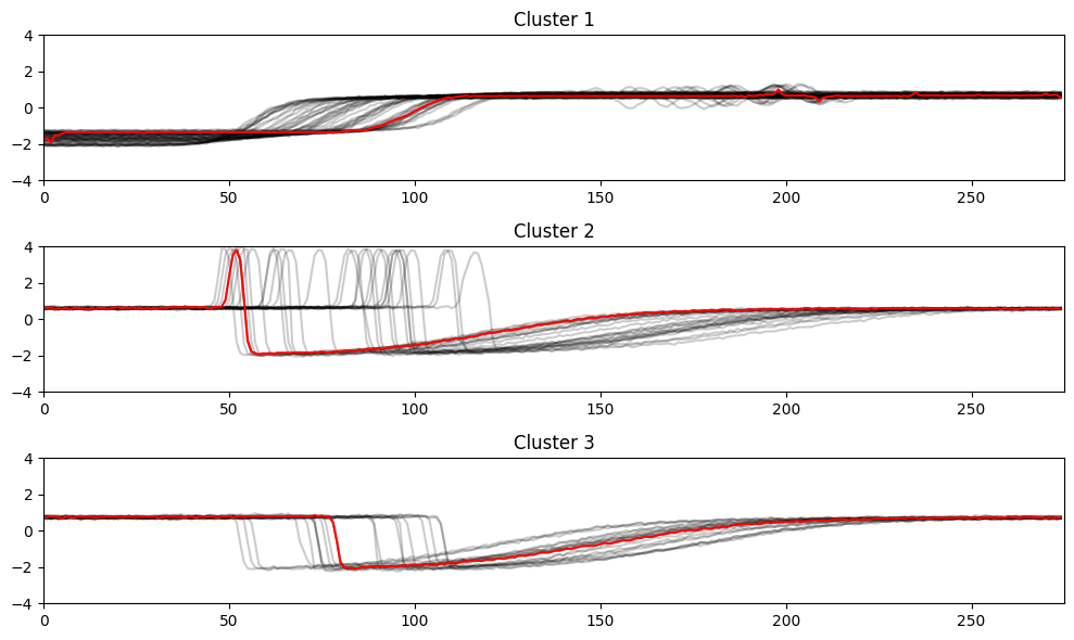
Graph Plot Of Time Series Dataset

Preprocessing techniques for time-series data

Preprocessing approaches for time-series data using similarity search mainly entail changing the time-series data into a format that can be effectively searched and compared. The following are some typical preparation strategies for time-series data using similarity search:

1. Discretization: The process of transforming continuous time-series data into a set of discrete values is known as discretization. This can be accomplished through the use of methods such as binning and quantization. Discretization can assist in reducing the dimensionality of time-series data, making it more suitable for similarity searches.
2. Normalization: Normalization is the process of adjusting time-series data to have a mean of zero and a standard deviation of one. Normalization can aid in reducing the impact of outliers in data and making it more similar across time series.
3. Dimensionality Reduction: Dimensionality reduction methods such as Principal Component Analysis (PCA) or Singular Value Decomposition (SVD) can be used to minimize the number of dimensions in time-series data. This can assist to accelerate similarity searches and minimize data storage needs.
4. Feature Extraction: Identifying relevant characteristics in time-series data that can be used to compare different time series is what feature extraction is all about. This may be accomplished with techniques such as the Fourier Transform or the Wavelet Transform. Feature extraction can aid in reducing data dimensionality and improving the accuracy of similarity searches.
5. Indexing: Indexing is the process of arranging time-series data into a searchable form. This may be accomplished through the use of techniques such as B-Trees or Hashing. Indexing can assist in reducing the time necessary to do a similarity search on time-series data.

Generally, similarity search preparation strategies for time-series data strive to reduce the dimensionality of the data, improve its comparability, and make it easier to search.

Applications of similarity search in time-series analysis

Time-series analysis makes extensive use of similarity search tools. Following are some applications for similarity search:

1. Anomaly detection: With time-series data, a similarity search may be used to find odd or aberrant patterns. It is feasible to find variations that may suggest an anomaly by comparing a new time series to a collection of reference time series. In the context of network security, for example, a similarity search can be used to discover unusual traffic patterns that may suggest a cyber assault.
2. Clustering: Similarity search may also be used to group comparable patterns in time series data. It is feasible to group people with similar features by comparing the similarity of each pair of time series. This can be beneficial for detecting trends in enormous datasets, such as financial or medical data analysis.
3. Forecasting: Similarity search may be used to find patterns in past time series data that can be used to predict future values. By comparing the similarity of a new time series to past data, trends, and patterns that may be utilized for forecasting can be identified. This may be beneficial in a variety of fields, including banking, weather forecasting, and energy use.

Ultimately, similarity search approaches have a wide variety of applications in time-series research, and they may be used to increase the accuracy and efficiency of various data analysis activities.

Challenges in similarity search

• Managing Missing Data: Missing values in time series data are common owing to a variety of factors such as sensor failures or data transmission issues. Missing data might impair similarity search results and make proper time-series data comparison difficult. As a result, efficient approaches for dealing with missing data are necessary.
• Managing vast and complicated data sets: Time-series data can be big and complicated, making typical methods difficult to handle and compare. Large data sets need effective indexing and search algorithms capable of swiftly identifying pertinent data pieces.
• Managing Time Shifts: Temporal shifts in time-series data can occur for a variety of reasons, including time zone variations or changes in data collecting periods. It is critical for reliable similarity search results to detect and rectify temporal shifts.
• High-resolution scaling: Time-series data might have many dimensions, making it difficult to look for comparable patterns in high-dimensional space. Traditional methods’ performance can decline quickly as the number of dimensions rises, making it difficult to handle high-dimensional data.
• Choosing the Best Similarity Measures: The accuracy of the similarity search results is affected by the choice of a suitable similarity measure in time-series analysis. Various similarity metrics are appropriate for different types of data, and choosing the proper one is critical for producing accurate and useful findings.

In summary, similarity search in time-series analysis has various problems that must be overcome to produce reliable and efficient findings. Some of the primary obstacles that must be solved to achieve successful similarity search in time-series research are effective management of missing data, dealing with vast and complicated data sets, selecting appropriate similarity measures, scaling to high dimensions, and addressing temporal changes.

Tools and libraries (In Python, C++, R & Java)

1. The R package “dtw”: Dynamic Time Warping (DTW) is a popular approach for determining the similarity of time series data. The R package “dtw” implements DTW for time-series analysis quickly and efficiently. It contains DTW computation methods such as the Sakoe-Chiba band and the Itakura parallelogram.
2. Python library “tslearn”: “tslearn” is a Python package that includes time-series analysis tools such as similarity measurements, clustering techniques, and classification methods. It comprises Euclidean distance, Dynamic Time Warping, and Edit Distance with Real Penalty implementations, among others.
3. Java library “MSTUMP”: “MSTUMP” is a Java package that provides a quick and scalable approach for constructing matrix profiles, a valuable tool for detecting patterns and abnormalities in time-series data. It contains distance metrics such as Euclidean and Manhattan distances.
4. Python library “pyts”: “pyts” is a Python package that includes dimensionality reduction methods, feature extraction algorithms, and distance measurements for time-series analysis. It comprises Euclidean distance, Dynamic Time Warping, and Edit Distance with Real Penalty implementations, among others.
5. C++ library “FLANN”: FLANN (Fast Library for Approximate Nearest Neighbors) is a C++ package that provides efficient methods for searching for nearest neighbors in high-dimensional space. It employs several indexing structures, including KD-trees, hierarchical clustering, and Locality-Sensitive Hashing (LSH).

To summarize, several strong tools and libraries are available for doing similarity searches in time-series research. Some of the prominent tools and libraries used by academics and developers in the field of time-series analysis include the “dtw” R package, the “tslearn” Python library, the “MSTUMP” Java library, the “pyts” Python library, and the “FLANN” C++ library.

Moreover, similarity search is an important element of time-series research that includes identifying patterns and trends in huge datasets. We reviewed many strategies for similarity search in this post, including Euclidean distance, Dynamic Time Warping, and Fourier Transform. We also investigated several applications of similarity search, such as data compression, anomaly detection, and classification.

The usefulness of similarity search in time-series analysis stems from its capacity to discover hidden insights and detect patterns that may not be obvious at first glance. This helps businesses to make more informed decisions, streamline operations, and improve overall performance. With the rising availability of time-series data in a variety of fields, efficient similarity search algorithms are more important than ever.

As a result, enterprises must invest in tools and methodologies that can execute accurate and quick similarity searches on massive datasets. This will provide them with a competitive advantage and boost their capacity to derive important insights from data.