Periodicity in Time Series Data using R

Periodicity refers to the existence of repeating patterns or cycles in the time series data. Periodicity helps users to understand the underlying trends and make some predictions which is a fundamental task in various fields like finance to climate science.

In time series data, the R Programming Language and its environment for statistical analysis offer a wide range of useful tools and techniques to explore periodicity. Now, we will explore the key functions, libraries, and visualization methods by using R programming language which can help to resolve the uncover hidden patterns in time series data.

What is Periodicity?

Periodicity is a fundamental characteristic of time series data in a program which refers to the regular repetition of patterns at fixed intervals. Periodicity means that something repeats after fixed intervals. These regular repetitions of patterns can occur daily, weekly, monthly basis or at any other consistent time interval.

For example, daily traffic patterns and weekly TV programs all present certain periodic patterns.

Required Tools for Analyzing Periodicity in R

We need to work with the time series data before analyzing periodicity. For handling the time series data R provides various types of packages like “zoo“, “tsibble” and “xts” which offer convenient data structures and methods for time series manipulation.

Identifying and handling periodicity is crucial in time series analysis for:

• Accurate modelling and forecasting
• Understanding seasonal patterns
• Detecting anomalies

Detecting Periodicity in R

R is one of the powerful tools which is used to analyze the data, R provides various functions to analyze and visualize the data. In this article, we will mainly focus on the Autocorrelation, Periodogram and Fast Fourier Transform to identify the periodic patterns in the data and ggplot2 to visualize the time series data.

R packages for Handling Periodicity:

xts:

• Creates and Handles the time series objects
• periodicity() function estimates periodicity
• apply.weekly(), apply.monthly(), etc., apply functions over periods
• Visualize periodicity using plot(): xts plot periodicity: path/to/plot_xts_periodicity.png

zoo:

• it is also similar to xts, but it has different object structure
• this package offers various functions to estimate the periodicity

partsm:

• this package is specifically designed for periodic autoregressive (PAR) models
• It tests for periodicity also fits the PAR models and also it performs the forecasting

Finding Patterns with R Functions

periodicity()

• It is a function from the xts package that is used to estimate the periodicity of a time series object.
• It works by calculating the median time between observations.
• It will return a list with information about the estimated periodicity Including :

1. difftime: The median time between observations
2. scale: A string describing the periodicity (e.g., “daily”, “weekly”, “monthly”, etc.).

Creating Synthetic Time Series Data

R

# Create a synthetic time series with high periodicity
set.seed(123)
n <- 120
time <- seq(1, n)
periodicity <- 12  # Monthly periodicity
amplitude <- 50
noise <- rnorm(n, mean = 0, sd = 10)
time_series <- amplitude * sin(2 * pi * (time - 1) / periodicity) + noise
head(time_series)

Output:

[1] -5.604756 22.698225 58.888353 50.705084 44.594148 42.150650

Plot the synthetic time series

R

# Plot the synthetic time series
plot(time_series, type = "l",
     main = "Time Series",
     xlab = "Time", ylab = "Values")

Output:

Time Series plot

The plot visually conveys how the synthetic time series values change over time, with a focus on highlighting the periodic nature of the data. Peaks and troughs in the line indicate the periodic cycles generated by the sinusoidal function, and you should observe a repeating pattern approximately every 12 time points (monthly periodicity).

Autocorrelation Function (ACF)

R

# Autocorrelation Function (ACF)
acf_result <- acf(time_series, main = "Autocorrelation Function")

Output:

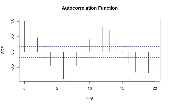
Autocorrelation Function

The ACF plot helps us identify the presence of periodic patterns in the data and provides insights into the cyclic behavior of the time series. In the case of high periodicity, you should observe significant peaks at multiples of the period, indicating a repeating pattern.

Periodogram

R

# Periodogram
spectrum(time_series, main = "Periodogram")

Output:

Periodogram

The periodogram is a useful for frequency analysis, and in the case of a time series with high periodicity, it should exhibit clear peaks at the frequencies associated with the periodic patterns in the data.

R

# Fast Fourier Transform (FFT)
fft_result <- fft(time_series)
plot(Mod(fft_result), main = "FFT Plot")

Output:

Fast Fourier Transform (FFT)

The FFT plot is another tool for frequency analysis, and it complements the information provided by the periodogram. Peaks in the FFT plot help pinpoint the frequencies associated with periodic patterns in the time series.

In this examples, we have created a synthetic time series data and demonstrate how to check the periodicity by performing Autocorrelation, Periodogram and Fast Fourier Transform . The final plot compares the original and imputed values.