Multi-Label Image Classification – Prediction of image labels
Last Updated :
26 Oct, 2021
There are so many things we can do using computer vision algorithms:
- Object detection
- Image segmentation
- Image translation
- Object tracking (in real-time), and a whole lot more.
What is Multi-Label Image Classification?
Let’s understand the concept of multi-label image classification with an intuitive example. If I show you an image of a ball, you’ll easily classify it as a ball in your mind. The next image I show you are of a terrace. Now we can divide the two images in two classes i.e. ball or no-ball.
When we have only two classes in which the images can be classified, this is known as a binary image classification problem.
- When there are more than two categories in which the images can be classified.
- An image does not belong to more than one category
If both of the above conditions are satisfied, it is referred to as a multi-class image classification problem.
Prerequisites:
Let’s start with some pre-requisites:
Here, we will be using the following languages and editors:
- Language/Interpreter : Python 3 (preferably python 3.8) from python.org
- Editor : Jupyter iPython Notebook
- OS : Windows 10 x64
- DataSet: Please download any image dataset from Kaggle or Internet.
- Python Requirements :This project requires the following libraries to be installed via pip: Numpy, Pandas, MatPlotLib, Scikit Learn, Scikit Image.
In the CMD window, run the following command to install the requirements:
—————————————————————————-
| pip install numpy pandas matplotlib notebook scikit-image scikit-learn |
—————————————————————————-
Note : replace pip with conda if you use anaconda!!
Now run jupyter and open the notebook in the files you downloaded earlier.
Steps to be followed:
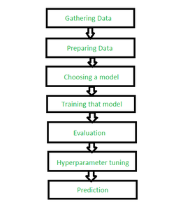
Steps for label classification
Step 1: Importing the libraries we need.
python3
import os
import warnings
warnings.simplefilter('ignore')
import numpy as np
import pandas as pd
import matplotlib.pyplot as plt
% matplotlib inline
from skimage.io import imread, imshow
from skimage.transform import resize
from skimage.color import rgb2grey
|
Step 2: Reading of target images into the project
In this portion of the article, we will be instructing python to read images one by one and then insert the pixel data of the images into arrays that we can use. Then we’ll be creating file lists by Python’s os library.
os.listdir(path) returns a list containing the names of the entries in the directory given by path.
python3
r = os.listdir(r"C:\Users\Garima Singh\Desktop\data\mugshots\r")
v = os.listdir(r"C:\Users\Garima Singh\Desktop\data\mugshots\v")
d = os.listdir(r"C:\Users\Garima Singh\Desktop\data\mugshots\d")
print(r[0:10])
|
Step 3: Creating and importing data from the images and Setting up a limit.
Here, we will use NumPy and scikit-image’s imread function. Since we have the downloaded data, we can quickly count how many images per subject we have. For example, suppose you have 100 images in each folder (r, v and d), you can set a variable limit with values 100. Next step is to create empty arrays for this data and filling up these arrays with data. We will quickly make 3 arrays to accommodate the data of the series of images. We create an array filled with “None” values using the following code snippet:
python3
limit = 100
ra_images = [None]*limit
i, j = 0, 0
for i in r:
if(j<limit):
ra_images[j] = imread(r"C:\Users\data\mugshots\r\\" + i)
j+= 1
else:
break
|
Step 4: Assembly of Data set and Flattening and reshaping of the arrays.
In this section, we will be using pandas Data Frame to merge these 3 data arrays into a single data array. Right now our image array is of size 28×28. We need to make this array into an array of 28^2 x 1. This basically means we have to make take each image and convert it into a row of data in our dataset.
python3
number_of_columns = ra_grey[1].shape[0] * ra_grey[1].shape[1]
print(number_of_columns)
|
Step 5: Flattening and Reshaping the data.
This is the part of the code that first converts the 28×28 array into a column vector (i.e. 784 x 1 matrix).
python3
print(ra_grey[0].shape)
for i in range(limit):
ra_grey[i] = np.ndarray.flatten(ra_grey[i]).reshape(number_of_columns, 1)
print(ra_grey[0].shape)
ra_grey = np.dstack(ra_grey)
print(ra_grey.shape)
ra_grey = np.rollaxis(ra_grey, axis = 2, start = 0)
print(ra_grey.shape)
ra_grey = ra_grey.reshape(limit, number_of_columns)
print(ra_grey.shape)
|
Doing the above for the rest of the data i.e. do the above 2 steps for the next 2 arrays.
Step 6: Converting arrays to dataframes
As discussed before, pandas makes a spreadsheet software like environment for our tables. Lets convert our arrays to dataframes:
python3
ra_data = pd.DataFrame(ra_grey)
dh_data = pd.DataFrame(dh_grey)
vi_data = pd.DataFrame(vi_grey)
ra_data
print(ra_data)
|
Step 7: Adding a name to the images.
In this step we add a column containing the name of our subjects.
This is called labelling our images. The model will try to predict based on the values and it will output one of these labels.
python3
ra_data["label"]="R"
dh_data["label"]="D"
vi_data["label"]="V"
vi_data
act = pd.concat([ra_data, dh_data])
actor = pd.concat([act, vi_data])
actor
|
Step 8: Shuffling the data and Printing the final data set
This is the last stage of this section. We will be shuffling the data, so that it may seem mixed.
python3
from sklearn.utils import shuffle
out = shuffle(actor).reset_index()
out
out = out.drop(['index'], axis = 1)
out
|
Step 9: Coding the machine learning algorithm + Testing Accuracy.
In this section we will code in the machine learning algorithm and find out our algorithm’s accuracy.
python3
x = out.values[:, :-1]
y = out.values[:, -1]
print(x[0:3])
print(y[0:3])
|
Step 10: Importing ML libraries and ML Coding
We will import a few ML libraries, all of these will come from sklearn and its classes.
python3
from sklearn.decomposition import PCA
from sklearn.svm import SVC
from sklearn.pipeline import make_pipeline
from sklearn.model_selection import train_test_split
from sklearn.model_selection import GridSearchCV
from sklearn import metrics
x_train, x_test, y_train, y_test = train_test_split(x, y, random_state = 0)
pca = PCA(n_components = 150, whiten = True, random_state = 0)
svc = SVC(kernel ='rbf', class_weight ='balanced')
model = make_pipeline(pca, svc)
params = {'svc__C': [x for x in range(1, 6)],
'svc__gamma': [0.001, 0.005, 0.006, 0.01, 0.05, 0.06, 0.004, 0.04]}
grid = GridSearchCV(model, params)
% time grid.fit(x_train, y_train)
print(grid.best_params_)
model = grid.best_estimator_
ypred = model.predict(x_test)
ypred[0:3]
|
We will use the PCA class and SVC class to create our model object. The make_pipeline will help us create an easy model that can be tested by GridSearchSV.
GridSearchSV is the function that will create a model with all of the parameters in EVERY combination possible and tell us which is the best combination.
Now that we have the model with the best parameters for our data, we use these parameters in our model and test its accuracy.
Step 11: Diagrams and getting accuracy
Lets see a visualized diagram of faces vs predicted labels:
python3
fig, ax = plt.subplots(4, 4, sharex = True,
sharey = True,
figsize = (10, 10))
for i, axi in enumerate(ax.flat):
axi.imshow(x_test[i].reshape(imsize).astype(np.float64),
cmap = "gray", interpolation = "nearest")
axi.set_title('Label : {}'.format(ypred[i]))
print(metrics.accuracy_score(y_test, ypred) * 100)
|
Conclusion:
Labeling the images to create the training data for machine learning or AI is not a difficult task. You just need the right techniques for it. This articles showed an image labeling process from scratch to mastery.
Share your thoughts in the comments
Please Login to comment...