Computing Classification Evaluation Metrics in R

Classification evaluation metrics are quantitative measures used to assess the performance and accuracy of a classification model. These metrics provide insights into how well the model can classify instances into predefined classes or categories.

The commonly used classification evaluation metrics are:

Confusion Matrix

It provides a detailed breakdown of the model’s predictions, enabling a more comprehensive understanding of its performance. The confusion matrix is particularly useful when evaluating classification problems with multiple classes.

A typical confusion matrix has two dimensions: the rows represent the actual class labels, and the columns represent the predicted class labels. Each cell in the matrix represents the count or frequency of instances that fall into a specific combination of actual and predicted classes.

The confusion matrix provides insights into the model’s performance for each class individually and overall. It helps identify the types of errors made by the model, such as false positives and false negatives. By analyzing the confusion matrix, practitioners can gain a deeper understanding of the model’s strengths and weaknesses and make informed decisions for model improvement and optimization. The confusion matrix allows for the calculation of various evaluation metrics:

• True Positives (TP): The instances that are correctly predicted as positive (actual positive, predicted positive).
• True Negatives (TN): The instances that are correctly predicted as negative (actual negative, predicted negative).
• False Positives (FP): The instances that are incorrectly predicted as positive (actual negative, predicted positive).
• False Negatives (FN): The instances that are incorrectly predicted as negative (actual positive, predicted negative).

Accuracy

Accuracy = (TP + FP) / (P + N)

Accuracy is a commonly used evaluation metric in classification tasks that measures the overall correctness of a model’s predictions. It provides a straightforward assessment of how well the model performs by calculating the ratio of correctly predicted instances to the total number of instances in the dataset.

Accuracy is easy to interpret and understand because it represents the proportion of correct predictions made by the model. However, it has limitations, especially in situations where the dataset is imbalanced or when misclassifying certain classes carries more significant consequences. Accuracy can be misleading when the classes in the dataset are imbalanced, meaning one class has significantly more instances than the others.

In such cases, a model that predicts the majority class for all instances would still achieve a high accuracy, but it may fail to perform well on the minority classes. Therefore, it is important to consider other evaluation metrics, especially when dealing with imbalanced datasets. Accuracy is a useful metric when misclassifying any class is equally important, and the class distribution is relatively balanced. For instance, in cases where the cost of false positives and false negatives is similar, accuracy provides a general overview of the model’s performance.

Precision

Precision = TP / (TP + FP)

Precision is an evaluation metric used in classification tasks that focuses on the correctness of positive predictions made by a model. It quantifies the proportion of correctly predicted positive instances out of all instances that are predicted as positive. In simpler terms, precision measures the ratio of the correctly identified positive instances (true positives) to the total number of instances that the model predicted as positive, regardless of whether the prediction was correct or incorrect.

For example, let’s say a model predicts 100 instances as positive. Out of those predictions, 80 are actually positive (true positives), but 20 are negative (false positives). In this case, the precision would be 80 / (80 + 20) = 0.8 or 80%. Precision is particularly useful when the cost or impact of false positive predictions is high. False positives occur when the model incorrectly identifies a negative instance as positive.

In scenarios where false positives have significant consequences, precision becomes a crucial metric to assess the model’s performance. For instance, in medical diagnosis, high precision is desirable because misclassifying a healthy patient as having a disease can lead to unnecessary treatments or procedures. In fraud detection, high precision is also desirable as misclassifying a legitimate transaction as fraudulent can cause inconvenience to the customer.

Recall (Sensitivity or True Positive Rate)

Recall = TP / (TP + FN)

Recall, also known as sensitivity or true positive rate, is an evaluation metric used in classification tasks to measure the model’s ability to correctly identify positive instances. It quantifies the proportion of true positive predictions out of all actual positive instances in the dataset. For example, let’s consider a binary classification problem where the model correctly identifies 80 positive instances out of a total of 100 actual positive instances. However, it fails to identify the remaining 20 positive instances (false negatives). In this case, the recall would be 80 / (80 + 20) = 0.8 or 80%.

A recall is particularly important in scenarios where the consequences of false negatives are high. False negatives occur when the model incorrectly predicts a positive instance as negative, which can result in missing critical instances or opportunities. A high recall is desired in certain domains, such as medical diagnosis or anomaly detection. In medical diagnosis, missing the identification of a disease can lead to delayed treatment or serious consequences. In anomaly detection, failing to identify abnormal events or patterns can lead to security breaches or operational failures.

F1 Score

F1 Score = (2 x Precision x Recall) / (Precision + Recall)

The F1 score is an evaluation metric used in classification tasks that provides a balanced measure of a model’s performance by taking into account both precision and recall. It is the harmonic mean of precision and recall, combining the two metrics into a single value. The F1 score ranges from 0 to 1, where a value of 1 represents perfect precision and recall, while a value of 0 indicates poor performance.

The F1 score is particularly useful when the dataset is imbalanced or when there is an uneven distribution between the positive and negative classes. It helps assess the model’s ability to achieve a balance between correctly identifying positive instances (precision) and capturing all actual positive instances (recall).The F1 score provides a single metric that balances precision and recall. It is useful when there is a trade-off between the two metrics, such as in situations where both false positives and false negatives are important.

In imbalanced datasets, where the majority class heavily outweighs the minority class, accuracy alone may not provide an accurate representation of the model’s performance. The F1 score considers both false positives and false negatives, making it a more reliable metric for evaluating the model’s effectiveness in such scenarios.

Specificity (True Negative Rate)

Specificity = TN / (TN + FP)

Specificity, also known as the true negative rate, is an evaluation metric used in binary classification tasks to measure a model’s ability to correctly identify negative instances. It quantifies the proportion of true negative predictions out of all actual negative instances in the dataset.

In simpler terms, specificity represents the ratio of correctly identified negative instances (true negatives) to the total number of instances that are actually negative, regardless of whether the model predicted them as negative or positive. For example, suppose we have a binary classification problem with 100 negative instances, out of which the model correctly identifies 80 as negative (true negatives) but incorrectly predicts 20 as positive (false positives). In this case, the specificity would be 80 / (80 + 20) = 0.8 or 80%.

Specificity is particularly important in scenarios where the cost or impact of false positive predictions is high. False positives occur when the model incorrectly predicts a negative instance as positive, which can result in unnecessary actions or consequences. In certain domains, such as medical screenings or quality control, a high specificity is desirable. In medical screenings, a high specificity ensures that healthy individuals are correctly identified as negative, reducing the chances of unnecessary tests or treatments. In quality control, a high specificity ensures that products meeting the required standards are not mistakenly classified as defective.

Kappa score

Kappa = (observed - expected) / (100% - expected)

Kappa score, also known as Cohen’s kappa coefficient, is an evaluation metric used in machine learning and statistics to measure the level of agreement between the predicted and actual class labels beyond what would be expected by chance. It is particularly useful when dealing with imbalanced datasets or when the class distribution is not uniform.

The kappa score ranges from -1 to 1, with 1 indicating perfect agreement, 0 indicating agreement by chance, and negative values indicating agreement worse than chance.

The kappa score is commonly used in situations where the class distribution is imbalanced or when there is a significant class skew. It provides a more robust measure of agreement by taking into account the agreement that can be expected by chance.

We will use the “iris” dataset for the programming example. It contains three categories of 50 instances each. We will use the random forest to classify the data into categories and then print the above-mentioned evaluation metrics in R.

Evaluation metrics in R

Step 1: Loading the necessary package

You can use various packages and functions to compute classification evaluation metrics in R. One commonly used package is “caret,” which provides a unified interface for many machine learning tasks, including evaluation.

Install the “caret” package, which stands for Classification And REgression Training. The “caret” package is a comprehensive framework in R for performing machine learning tasks, including data preprocessing, model training, and evaluation. Load the “caret” package into the R environment so that its functions and capabilities can be used.

R

# Install the package caret
install.packages("caret")
# Load the package into R program
library(caret)

Step 2: Loading Dataset

For this example, we use the “iris” dataset. Load the “iris” dataset, which is a famous dataset included in R. It contains measurements of different features of iris flowers (sepal length, sepal width, petal length, petal width) along with their corresponding species (setosa, versicolor, virginica).

Print a summary of the “iris” dataset, providing descriptive statistics such as mean, median, minimum, maximum, and quartiles for each feature.

R

# Load the dataset iris
data(iris)
# Print the summary of the dataset with summary function
summary(iris)

Output:

  Sepal.Length    Sepal.Width     Petal.Length    Petal.Width          Species  
 Min.   :4.300   Min.   :2.000   Min.   :1.000   Min.   :0.100   setosa    :50  
 1st Qu.:5.100   1st Qu.:2.800   1st Qu.:1.600   1st Qu.:0.300   versicolor:50  
 Median :5.800   Median :3.000   Median :4.350   Median :1.300   virginica :50  
 Mean   :5.843   Mean   :3.057   Mean   :3.758   Mean   :1.199                  
 3rd Qu.:6.400   3rd Qu.:3.300   3rd Qu.:5.100   3rd Qu.:1.800                  
 Max.   :7.900   Max.   :4.400   Max.   :6.900   Max.   :2.500 

This code block creates a scatter plot matrix of the “iris” dataset. It shows pairwise scatter plots of each feature against other features, allowing us to visualize the relationships and distributions between variables.

R

# Plot Pairs Scatter plot
plot(iris)

Output:

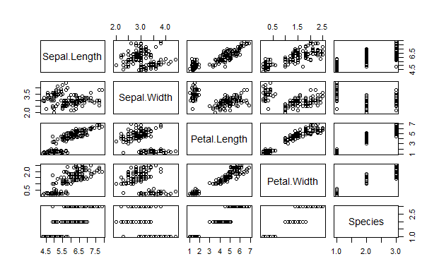
Pair plot

Uses the createDataPartition function from the “caret” package to split the data into a training set and a test set. It randomly selects 80% of the data for training by creating an index vector (trainIndex) that identifies the selected rows.

• iris$Species: This parameter specifies the target variable or outcome variable. In this case, it represents the species of the iris flowers.
• p: This parameter indicates the proportion of data to be allocated to the training set. In this example, it is set to 0.8, which means 80% of the data will be used for training.
• list: This parameter determines the format of the output. If list is set to FALSE, the function returns a numeric vector with the indices of the selected rows. If list is set to TRUE, it returns a list of indices for the selected rows.

Create two new datasets: trainData and testData. trainData contains 80% of the “iris” dataset, selected based on the trainIndex, while testData contains the remaining 20% of the dataset.

R

# Find the index of data with 80% split in matrix format
trainIndex <- createDataPartition(iris$Species, p = 0.8, list = FALSE)
# Store the 80% in trainData
trainData <- iris[trainIndex, ]
# Remaining 20% in testData
testData <- iris[-trainIndex, ]

Step 4: Model training

Installs the “randomForest” package, which provides the functionality to build random forest models. Random forests are an ensemble learning method that combines multiple decision trees to make predictions.

Use the train function from the “caret” package to train a classification model using the random forest method (method = "rf"). The formula Species ~ . specifies that the target variable is “Species,” and the remaining columns in the trainData dataset are used as predictors. The trained model is stored in the model variable.

• Species ~ .: This formula specifies the relationship between the target variable (Species) and the predictor variables. The ~ symbol separates the target variable from the predictors, and the . indicates that all other columns in the dataset (trainData) are used as predictors.
• data: This parameter specifies the training dataset on which the model will be trained. In this case, it is trainData.
• method: This parameter indicates the machine learning algorithm or method to be used for training the model. In this example, “rf” refers to the random forest algorithm.

R

# Install random forest library
install.packages("randomForest")

# load library
library(randomForest)

# Train a classification model
model <- train(Species ~ ., data = trainData, method = "rf")

Step 5: Evaluating Metrics

To calculate the evaluation metrics, test the model on the test data and save the answer in the predictions variable. use the confusionMatrix function from the “caret” package to calculate the confusion matrix and related metrics for the trained model’s predictions. The predictions argument should contain the predicted values, and testData$Species contains the actual species values from the test dataset. The resulting confusion matrix is stored in the cm variable.

• predictions: This parameter represents the predicted values obtained from the trained model. It should be a vector or factor containing the predicted class labels.
• testData$Species: This parameter provides the actual class labels from the test dataset. It represents the ground truth or true labels against which the predictions are compared.

R

# Make predictions on the test set
predictions <- predict(model, newdata = testData)
# Use the confusionmatrix function and pass in the predicted and real test values
cm<-confusionMatrix(predictions, testData$Species)

cm

Output:

Confusion Matrix and Statistics

            Reference
Prediction   setosa versicolor virginica
  setosa         10          0         0
  versicolor      0         10         1
  virginica       0          0         9

Overall Statistics
                                          
               Accuracy : 0.9667          
                 95% CI : (0.8278, 0.9992)
    No Information Rate : 0.3333          
    P-Value [Acc > NIR] : 2.963e-13       
                                          
                  Kappa : 0.95            
                                          
 Mcnemar's Test P-Value : NA              

Statistics by Class:

                     Class: setosa Class: versicolor Class: virginica
Sensitivity                 1.0000            1.0000           0.9000
Specificity                 1.0000            0.9500           1.0000
Pos Pred Value              1.0000            0.9091           1.0000
Neg Pred Value              1.0000            1.0000           0.9524
Prevalence                  0.3333            0.3333           0.3333
Detection Rate              0.3333            0.3333           0.3000
Detection Prevalence        0.3333            0.3667           0.3000
Balanced Accuracy           1.0000            0.9750           0.9500

Now the confusion matrix function results are stored in variable cm. We can access the accuracy, kappa, etc scores by using the argument overall to the variable cm. The overall metrics the measure the correctness or any other evaluation by using whole data and not separated by class i.e. it considers the whole result and not restricted by categories or not influenced by classes are shown in it.

To see the overall evaluation metrics use $overall and to see the classwise evaluation metrics use $byClass

R

cm$byClass

,

                  Sensitivity Specificity Pos Pred Value Neg Pred Value Precision
Class: setosa             1.0        1.00      1.0000000       1.000000 1.0000000
Class: versicolor         1.0        0.95      0.9090909       1.000000 0.9090909
Class: virginica          0.9        1.00      1.0000000       0.952381 1.0000000
                  Recall        F1 Prevalence Detection Rate Detection Prevalence
Class: setosa        1.0 1.0000000  0.3333333      0.3333333            0.3333333
Class: versicolor    1.0 0.9523810  0.3333333      0.3333333            0.3666667
Class: virginica     0.9 0.9473684  0.3333333      0.3000000            0.3000000
                  Balanced Accuracy
Class: setosa                 1.000
Class: versicolor             0.975
Class: virginica              0.950

As you can see above, we get all the classwise evaluation scores. From this, we can observe the sensitivity, Specificity, Precision, Recall, and F1 Score.

R

cm$overall

Output:

      Accuracy          Kappa  AccuracyLower  AccuracyUpper   AccuracyNull 
  9.666667e-01   9.500000e-01   8.278305e-01   9.991564e-01   3.333333e-01 
AccuracyPValue  McnemarPValue 
  2.962731e-13            NaN 

The cm$byClass line retrieves the performance metrics (such as accuracy, precision, recall, and F1 score) for each class separately. The cm$overall the line provides overall performance metrics across all classes.

Example 2:

To demonstrate classification evaluation metrics on a generated dataset in R, let’s walk through an example step-by-step:

Step 1: Generate a synthetic dataset with a factor outcome variable

In this step, we generate a synthetic binary classification dataset with 1000 samples. The dataset consists of 5 numerical features (features) and a binary class label (labels).

R

# Set the random seed for reproducibility
set.seed(123)

# Generate a binary classification dataset with 1000 samples
n <- 1000
features <- matrix(rnorm(n * 5), ncol = 5)
labels <- factor(sample(c(0, 1), n, replace = TRUE))
dataset <- data.frame(features, labels)

• set.seed(123): This line sets the random seed to 123, ensuring the reproducibility of the random numbers generated.
• n <- 1000: This line sets the number of samples to 1000.
• features <- matrix(rnorm(n * 5), ncol = 5): This line generates a matrix of random numbers using the rnorm function from a standard normal distribution. The matrix has n rows (1000 in this case) and 5 columns.
• labels <- factor(sample(c(0, 1), n, replace = TRUE)): This line creates a factor variable labels by randomly sampling 0s and 1s with replacement from the vector c(0, 1) using the sample function. The resulting labels variable represents the class labels for the binary classification problem.
• dataset <- data.frame(features, labels): This line combines the features matrix and the labels variable to create a data frame dataset that represents the synthetic dataset.

Step 2: Split the dataset into training and test sets

Here, we use the createDataPartition function to split the dataset into an 80% training set (trainData) and a 20% test set (testData).

R

# Split the dataset into 80% training and 20% test
trainIndex <- createDataPartition(dataset$labels, p = 0.8, list = FALSE)
trainData <- dataset[trainIndex, ]
testData <- dataset[-trainIndex, ]

• trainIndex <- createDataPartition(dataset$labels, p = 0.8, list = FALSE): This line uses the createDataPartition function from the “caret” package to split the dataset into a training set and a test set.
  • dataset$labels: This parameter specifies the outcome variable (class labels) of the dataset (dataset) that we want to split.
  • p = 0.8: This parameter specifies the proportion of the dataset that should be allocated to the training set. In this case, 80% of the data will be assigned to the training set.
  • list = FALSE: This parameter indicates whether the output should be returned as a list or not. By setting it to FALSE, the function returns a vector of indices indicating the selected samples for the training set.
• trainData <- dataset[trainIndex, ]: This line creates the training dataset (trainData) by subsetting the original dataset (dataset) using the indices specified by trainIndex. It selects the rows in dataset corresponding to the indices in trainIndex.
• testData <- dataset[-trainIndex, ]: This line creates the test dataset (testData) by subsetting the original dataset (dataset) using the complement of the indices in trainIndex. It selects the rows in dataset that are not included in the training set.

The createDataPartition the function ensures that the splitting of the dataset is randomized and maintains the proportion of class labels in both the training and test sets.

Step 3: Train a classification model

In this step, we train a logistic regression model using the train function from the “caret” package. The formula labels ~ . specifies the relationship between the target variable (labels) and the predictor variables. The method = "glm" parameter indicates the use of generalized linear modeling and family = "binomial" specifies that the logistic regression model is used for binary classification.

R

# Train a logistic regression model
model <- train(labels ~ ., data = trainData,
               method = "glm", family = "binomial")

The parameters used are as follows:

• model <- train(labels ~ ., data = trainData, method = "glm", family = "binomial"): This line trains a logistic regression model using the train function from the “caret” package.
  • labels ~ .: This formula specifies the relationship between the target variable (labels) and the predictor variables. The ~ symbol separates the target variable from the predictors. In this case, . represents all the other variables in the dataset (trainData) as predictors.
  • data = trainData: This parameter specifies the training dataset (trainData) from which the model will learn the relationships between the predictors and the target variable.
  • method = "glm": This parameter specifies the method for training the model. In this case, “glm” refers to the generalized linear modeling approach, which is used for logistic regression.
  • family = "binomial": This parameter specifies the family of the generalized linear model. For binary classification problems, the binomial family is commonly used, as it is suitable for modeling binary outcomes.

The train function is a part of the “caret” package, and it automatically selects the appropriate algorithm and performs the training based on the specified method and model formula.

Step 4: Make predictions on the test set

Here, we use the trained model to make predictions on the test set (testData) using the predict function. The predicted labels are stored in the predictions variable.

R

# Make predictions on the test set
predictions <- predict(model, newdata = testData)

Parameters used are as follows:

• predictions <- predict(model, newdata = testData): This line uses the predict function to make predictions on the test set (testData) using the trained classification model (model).
  • model: This parameter specifies the trained model object from which predictions will be made.
  • newdata = testData: This parameter specifies the new data on which the predictions will be made. In this case, the test dataset (testData) is used as the new data.

The predict function takes the trained model and applies it to the test dataset to generate predictions. The resulting predictions are stored in the predictions variable

Step 5: Evaluate the model using classification evaluation metrics

In this step, we evaluate the trained model’s performance using various classification evaluation metrics:

• Confusion Matrix: The confusionMatrix function calculates the confusion matrix, which provides a summary of the model’s predictions compared to the true labels.
• Accuracy: The overall accuracy of the model is computed as the proportion of correct predictions (both true positives and true negatives) out of the total predictions.
• Precision: Precision, also known as the positive predictive value, measures the proportion of correctly predicted positive instances (true positives) out of the total predicted positive instances (true positives + false positives).
• Recall (Sensitivity or True Positive Rate): Recall, also known as sensitivity or true positive rate, measures the proportion of correctly predicted positive instances (true positives) out of the total actual positive instances (true positives + false negatives).
• F1 Score: The F1 score is the harmonic mean of precision and recall. It provides a single metric that balances precision and recall, giving equal importance to both. The F1 score ranges from 0 to 1, where a higher value indicates better performance.

R

# Calculate the confusion matrix
cm <- confusionMatrix(predictions, testData$labels)

# Print by class metrics
cm$byClass

#Print the overall metrics
cm$overall

Output:

> cm$byClass
         Sensitivity          Specificity       Pos Pred Value 
           0.5544554            0.3979592            0.4869565 
      Neg Pred Value            Precision               Recall 
           0.4642857            0.4869565            0.5544554 
                  F1           Prevalence       Detection Rate 
           0.5185185            0.5075377            0.2814070 
Detection Prevalence    Balanced Accuracy 
           0.5778894            0.4762073 
> #Print the overall metrics
> cm$overall
      Accuracy          Kappa  AccuracyLower  AccuracyUpper   AccuracyNull 
    0.47738693    -0.04768654     0.40627445     0.54918310     0.50753769 
AccuracyPValue  McnemarPValue 
    0.82164281     0.20239602 

cm$byClass refers to a component of the confusion matrix object (cm). It provides detailed performance metrics for each class in a multi-class classification problem.

cm$overall refers to a component of the confusion matrix object (cm). It provides an overall summary of performance metrics for the classification model.

This way we can calculate the different classification evaluation metrics in R by using just ‘caret’ library and creating a confusion matrix.