Leukaemia Cell Classification For Paediatric Cancer Diagnosis

In the world of children’s cancer, especially leukaemia, our focus is on using the latest technology to help battle pediatric cancer. We are using deep learning techniques to build a model that will increase the precision with which medical professionals identify childhood leukaemia.

Leukaemia Cell Classification For Paediatric Cancer Diagnosis

What is Pediatric cancer?

Pediatric cancer is a type of cancer specifically affecting children, characterized by the uncontrolled growth of abnormal white blood cells in the bone marrow. This condition compromises the production of healthy blood cells, leading to symptoms such as fatigue, infections, and bruising.

What is a Leukemia cell?

Leukaemia cells are aberrant blood cells that develop in the bone marrow and interfere with the normal synthesis of blood cells. They lead to symptoms such as exhaustion, infections, and bleeding.

Model Description:

In this article, we have created a Convolutional Neural Network (CNN) model that exhibits a hierarchical architecture for binary classification tasks, particularly suited for image-related applications.

It consists of two types of cell images :

• ALL (Cancer Cells): Acute lymphoblastic leukaemia cells are a kind of malignant cells that mostly impact white blood cells. This class represents these cells.
• HEM( Normal Cells): Normal hematopoietic cells, or healthy blood-forming cells present in the bone marrow, are referred to by this class.

We have to classify into two classes, thus we will use the sigmoid activation function in the output layer.

Prerequisites:

TensorFlow is an open-source machine learning framework. Various ecosystem of tools,libraries which help in optimisation of models are present in it.

!pip install tensorflow

OpenCV is an open-source computer vision and machine learning software library. It offers a varied range of functions for image and video processing.

!pip install opencv-python

Leukaemia Cell Classification For Paediatric Cancer Diagnosis Implementation:

Modify the file paths accordingly.

Import the necessary libraries

Python3

#importing necessary libraries
import os
import pandas as pd
import numpy as np
import matplotlib.pyplot as plt
import seaborn as sns
from sklearn.model_selection import train_test_split
from sklearn.metrics import classification_report
from warnings import filterwarnings
filterwarnings('ignore')

import cv2 as cv
from PIL import Image
from tensorflow.keras.optimizers import Adam
from keras import optimizers
from keras.models import Sequential
from keras.regularizers import l2
from tensorflow.keras.optimizers import Adam
from keras.layers import Dense, Conv2D, Flatten, MaxPool2D, Dropout, BatchNormalization
from tensorflow.keras.callbacks import ModelCheckpoint

Define the general parameters for our model.

Python3

# General Params
MAIN_SEED = 42  # Random Seed
# For our CNN model
USE_LESS_DATA = True  # If not enough mem available
LR = 0.01  # Learning Rate
BATCH_SIZE = 32  # Batch Size
EPOCH = 10
IMAGE_RESIZE_X = 200  # Image Width
IMAGE_RESIZE_Y = 200  # Image height
KEEP_COLOR = False  # Keep color in images. Color takes 3x Mem space

• Then utilise an os.walk loop to efficiently traverses the specified directory, categorizing cell images into ‘hem’ (normal) and ‘all’ (leukaemia) based on folder names.

Python3

total_all_count = 0
total_hem_count = 0
for dirname, _, filenames in os.walk('.../C-NMC_Leukemia/training_data'):
    for filename in filenames:
        all_count = 0
        hem_count = 0
        if "training" in dirname:
            if "all" in dirname:
                all_count = len(filenames)
            elif "hem" in dirname:
                hem_count = len(filenames)
            total_all_count += all_count
            total_hem_count += hem_count
            break
print(
    f"HEM(Normal) Cell Count {total_hem_count} \nALL(Leukemia) Cell Count {total_all_count}")

Output:

HEM(Normal) Cell Count 3389 
ALL(Leukaemia) Cell Count 7272

Analysing distribution of Target class

• Matplotlib is used to create a bar plot representing the counts of ‘HEM – Normal’ and ‘ALL – Leukaemia’ classes in the training data, enhancing visualisation and understanding of the dataset distribution.

Python3

# Data
data = {'HEM - Normal':total_hem_count, 'ALL - Leukemia':total_all_count}
courses = list(data.keys())
values = list(data.values())

fig = plt.figure(figsize = (10, 5))

# creating the bar plot
plt.bar(courses, values, color ='navy')

plt.xlabel("Class")
plt.ylabel("Count")
plt.title("Target Class Distribution")
plt.show()

Output:

• Then the code utilizes the os module to explore and access directories, extracting a specific image path from a hierarchical file structure related to leukemia data. It then employs the PIL (Python Imaging Library) to open and load an image for further processing.

Data Loading

Python3

folder = '..../C-NMC_Leukemia'
print(os.listdir(folder))
train = os.path.join(folder,'training_data')

fold_0 =os.path.join(train,os.listdir(train)[0])

all_img_path = os.path.join(fold_0, os.listdir(fold_0)[-1])
img_path = os.path.join(all_img_path,os.listdir(all_img_path)[0])
img_path


img = Image.open(img_path)

Output:

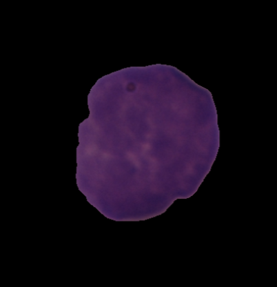
A sample image from dataset

• The code initializes two lists to store image paths and corresponding labels, iterates through specified folders containing leukemia data, and determines labels based on folder names (1 for ‘all’ and 0 for ‘hem’). It constructs full image paths and appends them, along with labels, to the respective lists. Finally, a Pandas DataFrame is created to organize the image paths and labels for further processing and analysis.

Python3

# Initialize lists to store image paths and labels
image_paths = []
image_labels = []

# Iterate through the specified folders
for data_folder_path in [training_all_0, training_all_1, training_all_2, training_hem_0, training_hem_1, training_hem_2]:
    all_images_in_folder = os.listdir(data_folder_path)

    # Determine the label based on the folder name
    image_label = 1 if 'all' in data_folder_path else 0

    # Iterate through images in the folder
    for image_path in all_images_in_folder:
        # Construct the full image path
        full_image_path = os.path.join(data_folder_path, image_path)

        # Append the image path and label to the lists
        image_paths.append(full_image_path)
        image_labels.append(image_label)

# Create a DataFrame from the lists
dict_train = {"image_paths": image_paths, "image_labels": image_labels}
df_train = pd.DataFrame(dict_train)

The code below uses Pandas to read a CSV file containing validation data, rename columns in the DataFrame, and add a new column for full image paths. Then we append the base path to construct complete image paths for further use in the validation dataset.

Python3

df_val = pd.read_csv('..../C-NMC_Leukemia/validation_data/C-NMC_test_prelim_phase_data_labels.csv')
# Drop Patient_ID column and rename columns
df_val['image_paths'] = df_val['new_names']
df_val['image_labels'] = df_val['labels']
df_val = df_val[['image_paths', 'image_labels']]

base_path = '..../C-NMC_Leukemia/validation_data/C-NMC_test_prelim_phase_data'
df_val['image_paths'] = df_val['image_paths'].apply(lambda x: os.path.join(base_path, x))

Data Preprocessing

• The provided below function, `read_and_crop_image`, reads an image using the PIL library, converts it to a NumPy array, and applies color system conversion from BGR to grayscale.
• We then employ Otsu’s thresholding for image segmentation, which crops the image based on the segmented region, and resizes it to a specified resolution. Additionally, the function includes options for maintaining color (`KEEP_COLOR`) and utilizes OpenCV for various image processing operations, such as thresholding, bitwise operations, and border padding.

Python3

def read_and_crop_image(image_path):
    # Read image using PIL
    img = Image.open(image_path)
    image = np.array(img)  # Convert PIL image to NumPy array

    # Convert Color System from BGR(Blue, Green, Red) to GRAY
    gray = cv.cvtColor(image, cv.COLOR_BGR2GRAY)

    # Apply Otsu's Thresholding
    thresh = cv.threshold(
        gray, 0, 255, cv.THRESH_BINARY_INV + cv.THRESH_OTSU)[1]

    # Apply threshold
    result = cv.bitwise_and(image, image, mask=thresh)
    result[thresh == 0] = [255, 255, 255]
    (x, y, z_) = np.where(result > 0)
    mnx = (np.min(x))
    mxx = (np.max(x))
    mny = (np.min(y))
    mxy = (np.max(y))

    # Crop Image
    crop_img = image[mnx:mxx, mny:mxy, :]

    # Resize image
    border_v = 0
    border_h = 0
    if (IMAGE_RESIZE_Y / IMAGE_RESIZE_X) >= (crop_img.shape[0] / crop_img.shape[1]):
        border_v = int((((IMAGE_RESIZE_Y / IMAGE_RESIZE_X) *
                         crop_img.shape[1]) - crop_img.shape[0]) / 2)
    else:
        border_h = int((((IMAGE_RESIZE_Y / IMAGE_RESIZE_X) *
                         crop_img.shape[0]) - crop_img.shape[1]) / 2)

    crop_img = cv.copyMakeBorder(
        crop_img, border_v, border_v, border_h, border_h, cv.BORDER_CONSTANT, 0)
    resized_image = cv.resize(crop_img, (IMAGE_RESIZE_X, IMAGE_RESIZE_Y))

    # Return colorful image if KEEP_COLOR set
    if KEEP_COLOR:
        return resized_image
    else:
        return cv.cvtColor(resized_image, cv.COLOR_BGR2GRAY)

• The code then applies our crop preprocessing function (`read_and_crop_image`) to extract features from image paths in the training and validation datasets. It stacks the processed images and corresponding labels, expands dimensions to add channel information if images are colorless, and splits the training data into training and testing sets using `train_test_split`. The output prints the shapes of the resulting arrays, providing a concise summary of the dataset dimensions.

Python3

#Applying Crop preprocess
X_train = df_train['image_paths'].apply(read_and_crop_image).values
X_val = df_val['image_paths'].apply(read_and_crop_image).values

y_train = df_train['image_labels'].values
y_val = df_val['image_labels'].values

X_train = np.stack(X_train, axis=0)
X_val = np.stack(X_val, axis=0)

#Expand dim to add channel info if image has 1 channel(Colorless)
if not KEEP_COLOR:
    X_train = np.expand_dims(X_train, axis=-1)
    X_val = np.expand_dims(X_val, axis=-1)

 X_train, X_test, y_train, y_test = train_test_split(X_train, y_train, test_size=0.1, random_state = MAIN_SEED)

print("X_train ->",X_train.shape,
      "\ny_train ->",y_train.shape,
      "\n\nX_test ->",X_test.shape,
      "\ny_test ->",y_test.shape,
      "\n\nX_val ->",X_val.shape,
      "\ny_val ->",y_val.shape
)

Output:

X_train -> (4050, 100, 100, 1) 
y_train -> (4050,) 
X_test -> (450, 100, 100, 1) 
y_test -> (450,) 
X_val -> (1000, 100, 100, 1) 
y_val -> (1000,)

Model Building

Now, we define our convolutional neural network (CNN) model using the Sequential API with layers for convolution, max pooling, dropout, flattening, dense, and batch normalization. It incorporates various hyperparameters such as filter size, kernel size, activation functions, and regularization.

Python3

model = Sequential()
model.add(Conv2D(filters=2, kernel_size=(3, 3), padding='valid', activation='relu', input_shape=input_shape))
model.add(Conv2D(filters=4, kernel_size=(3, 3), padding='valid', activation='relu'))
model.add(Conv2D(filters=8, kernel_size=(5, 5), padding='valid', activation='relu'))
model.add(MaxPool2D(pool_size=(2, 2)))
model.add(Dropout(0.5))

model.add(Conv2D(filters=16, kernel_size=(5, 5), padding='valid', activation='relu'))
model.add(MaxPool2D(pool_size=(2, 2)))
model.add(Flatten())

model.add(Dense(8, kernel_regularizer=l2(1e-5), activation="relu"))
model.add(BatchNormalization())

model.add(Dense(1, activation="sigmoid"))
model.summary()

Model: "sequential_11"
_________________________________________________________________
 Layer (type)                Output Shape              Param #   
=================================================================
 conv2d_46 (Conv2D)          (None, 98, 98, 2)         20        
                                                                 
 conv2d_47 (Conv2D)          (None, 96, 96, 4)         76        
                                                                 
 conv2d_48 (Conv2D)          (None, 92, 92, 8)         808       
                                                                 
 max_pooling2d_22 (MaxPooling (None, 46, 46, 8)         0         
 ng2D)                                                           
                                                                 
 dropout_22 (Dropout)        (None, 46, 46, 8)         0         
                                                                 
 conv2d_49 (Conv2D)          (None, 42, 42, 16)        3216      
                                                                 
 max_pooling2d_23 (MaxPooling  (None, 21, 21, 16)        0         
 ng2D)                                                           
                                                                 
 dropout_23 (Dropout)        (None, 21, 21, 16)        0         
                                                                 
 flatten_11 (Flatten)        (None, 7056)              0         
                                                                 
 dense_36 (Dense)            (None, 8)                 56456     
...
Total params: 60617 (236.79 KB)
Trainable params: 60601 (236.72 KB)
Non-trainable params: 16 (64.00 Byte)
_____________________________________________

Model Compilation

We create the model using binary cross entropy as the loss function for binary classification, configures the Adam optimizer with a given learning rate (0.01), and uses accuracy as the metric to track throughout training.

Python3

optimizer = Adam(lr=LR)
model.compile(optimizer=optimizer, loss='binary_crossentropy',
              metrics=['accuracy'])

Saving The Model

The filepath (‘best_model.h5’) to save the best model based on minimising validation loss is specified in a ModelCheckpoint callback that is defined. The callback stores only the model that performs the best while keeping an eye on ‘val_loss’. In order to save the optimal model weights, the ModelCheckpoint callback is integrated into the training process, after the model (model) is fitted to the training data with batch size, epochs, and validation data supplied.We get the highest model accuracy to be near about 70%.

Python3

# Define a ModelCheckpoint callback
checkpoint = ModelCheckpoint(
    'best_model.h5',  # Filepath to save the best model
    monitor='val_loss',  # Metric to monitor for improvement
    save_best_only=True,  # Save only the best model
    mode='min',  # 'min' for val_loss, 'max' for val_accuracy, etc.
    verbose=1  # 1: prints a message for each improvement
)

Train the model

Python3

# Train the model with ModelCheckpoint callback
model_trained = model.fit(
    X_train, y_train,
    batch_size=BATCH_SIZE,
    epochs=10,
    validation_data=(X_val, y_val),
    callbacks=[checkpoint]  # Add the ModelCheckpoint callback
)

Model Evaluations

• Two graphs are made: one shows the loss during training and validation over epochs, and the other shows the accuracy of the model throughout training and validation. Over the course of training, these visualisations shed light on the model’s performance and convergence.

Python3

# Creating subplots
plt.figure(figsize=(12, 6))

# Subplot for Loss
plt.subplot(1, 2, 1)
plt.plot(first_model_trained.history['loss'], label='Training Loss')
plt.plot(first_model_trained.history['val_loss'], label='Validation Loss')
plt.xlabel('Epoch')
plt.ylabel('Loss')
plt.title('Training and Validation Loss Over Epochs')
plt.legend()

# Subplot for Accuracy
plt.subplot(1, 2, 2)
plt.plot(first_model_trained.history['accuracy'], label='Training Accuracy')
plt.plot(
    first_model_trained.history['val_accuracy'], label='Validation Accuracy')
plt.title('Training and Validation Accuracy Over Epochs')
plt.ylabel('Accuracy')
plt.xlabel('Epoch')
plt.legend(loc='lower right')

# Adjusting layout to prevent overlap
plt.tight_layout()

# Displaying the plot
plt.show()

Output:

The graph may appear distorted or skewed due to the scaling of the x-axis.

Classifications Report

We defined folder_path for testing data, did all the preprocessing on the testing data like the training data , thenmade predictions on the reshaped data, and printed a classification report .

Python3

folder_path = '/Users/arundhutichakraborty/Downloads/C-NMC_Leukemia/testing_data/C-NMC_test_final_phase_data'
X_test = [read_and_crop_image(os.path.join(folder_path, filename))
          for filename in os.listdir(folder_path)]

# Convert the list of images to a NumPy array
X_test = np.stack(X_test, axis=0)
# Reshape the input data to match the model's input shape
X_test_reshaped = X_test.reshape(-1, 100, 100, 1)trained_model = first_model_trained.model

# Make predictions
predicted = trained_model.predict(reshaped_data)
target_names = ['HEM', 'ALL']

# Generate the classification report
print(classification_report(y_test, binary_predictions, target_names=target_names))

Output:

              precision    recall  f1score   support
         HEM       0.31      0.70      0.43       144
         ALL       0.66      0.27      0.38       306
    accuracy                           0.41       450
   macro avg       0.48      0.48      0.41       450
weighted avg       0.55      0.41      0.40       450

Predictions

Now, we define a function `predict_and_display`, which loads our trained model (`best_model.h5`), preprocesses an input image using a specified preprocessing function (`read_and_crop_image`), makes predictions, applies thresholding, and displays the original image with the prediction.

Python3

def predict_and_display(input_image_path, model_path='best_model.h5', threshold=0.5):
    # Load the trained model
    loaded_model = load_model(model_path)

    # Preprocess the input image
    input_image = read_and_crop_image(input_image_path)  # Use your image preprocessing function
    input_image = input_image / 255.0  # Assuming pixel values are in the range [0, 255]

    # Make predictions
    predictions = loaded_model.predict(np.expand_dims(input_image, axis=0))

    # Apply thresholding
    binary_predictions = np.where(predictions > threshold, 1, 0)

    # Display the image and predictions
    plt.imshow(input_image)
    if binary_predictions[0] == 1:
        plt.title('Prediction: ALL')
    else:
        plt.title('Prediction: 0')
    plt.show()

# Example usage
input_image_path = '/Users/arundhutichakraborty/Downloads/C-NMC_Leukemia/testing_data/C-NMC_test_final_phase_data/2.bmp'
predict_and_display(input_image_path)

Output:

A cell with prediction.