ML | Face Recognition Using PCA Implementation
Last Updated :
30 Nov, 2021
Face Recognition is one of the most popular and controversial tasks of computer vision. One of the most important milestones is achieved using This approach was first developed by Sirovich and Kirby in 1987 and first used by Turk and Alex Pentland in face classification in 1991. It is easy to implement and thus used in many early face recognition applications. But it has some caveats such as this algorithm required cropped face images with proper light and pose for training. In this article, we will be discussing the implementation of this method in python and sklearn.
We need to first import the scikit-learn library for using the PCA function API that is provided into this library.
The scikit-learn library also provided an API to fetch LFW_peoples dataset. We also required matplotlib to plot faces.
Code: Importing libraries
Python3
import matplotlib.pyplot as plt
from sklearn.model_selection import train_test_split
from sklearn.model_selection import GridSearchCV
from sklearn.datasets import fetch_lfw_people
from sklearn.metrics import classification_report
from sklearn.metrics import confusion_matrix
from sklearn.decomposition import PCA
from sklearn.svm import SVC
import numpy as np
|
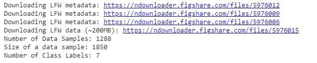
Now we import the LFW_people dataset using sklearn’s fetch_lfw_people function API. LFW_prople is the preprocess excerpt of LFW. It contains 13233 images of 5749 classes of shape 125 * 94. This function provides an parameter min_faces_per_person. This parameter allows us to select the classes that have at least min_faces_per_person different pictures. This function also has a parameter resize which resize every image in the extracted face. We use min_faces_per_person = 70 and resize = 0.4.
Code:
Python3
lfw_people = fetch_lfw_people(min_faces_per_person = 70, resize = 0.4)
n_samples, h, w = lfw_people.images.shape
X = lfw_people.data
n_features = X.shape[1]
y = lfw_people.target
target_names = lfw_people.target_names
n_classes = target_names.shape[0]
print("Number of Data Samples: % d" % n_samples)
print("Size of a data sample: % d" % n_features)
print("Number of Class Labels: % d" % n_classes)
|
Output:
Code: Data Exploration
Python3
def plot_gallery(images, titles, h, w, n_row = 3, n_col = 4):
plt.figure(figsize =(1.8 * n_col, 2.4 * n_row))
plt.subplots_adjust(bottom = 0, left =.01, right =.99, top =.90, hspace =.35)
for i in range(n_row * n_col):
plt.subplot(n_row, n_col, i + 1)
plt.imshow(images[i].reshape((h, w)), cmap = plt.cm.gray)
plt.title(titles[i], size = 12)
plt.xticks(())
plt.yticks(())
def true_title(Y, target_names, i):
true_name = target_names[Y[i]].rsplit(' ', 1)[-1]
return 'true label: % s' % (true_name)
true_titles = [true_title(y, target_names, i)
for i in range(y.shape[0])]
plot_gallery(X, true_titles, h, w)
|

Dataset Sample Images with True Labels
Now, we apply train_test_split to split the data into training and testing sets. We use 25% of the data for testing.
Code: Splitting the dataset
Python3
X_train, X_test, y_train, y_test = train_test_split(
X, y, test_size = 0.25, random_state = 42)
print("size of training Data is % d and Testing Data is % d" %(
y_train.shape[0], y_test.shape[0]))
|

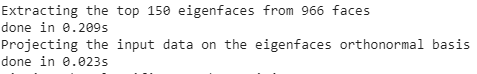
Now, we apply the PCA algorithm on the training dataset which computes EigenFaces. Here, we take n_components = 150 means we extract the top 150 Eigenfaces from the algorithm. We also print the time taken to apply this algorithm.
Code: Implementing PCA
Python3
n_components = 150
t0 = time()
pca = PCA(n_components = n_components, svd_solver ='randomized',
whiten = True).fit(X_train)
print("done in % 0.3fs" % (time() - t0))
eigenfaces = pca.components_.reshape((n_components, h, w))
print("Projecting the input data on the eigenfaces orthonormal basis")
t0 = time()
X_train_pca = pca.transform(X_train)
X_test_pca = pca.transform(X_test)
print("done in % 0.3fs" % (time() - t0))
|
The above code generates the EigenFace and each image is represented by a vector of size 1 * 150. The values in this vector represent the coefficient corresponding to that Eigenface. These coefficient are generated using transform function on the function.
Eigenfaces generated by this PCA algorithm:
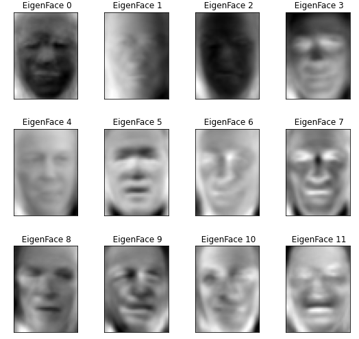
EigenFaces
Code: Explore the coefficient generated by the above algorithm.
Python3
print("Sample Data point after applying PCA\n", X_train_pca[0])
print("-----------------------------------------------------")
print("Dimensions of training set = % s and Test Set = % s"%(
X_train.shape, X_test.shape))
|
Sample Data point after applying PCA
[-2.0756025  -1.0457923   2.126936    0.03682641 -0.7575693  -0.51736575
  0.8555038   1.0519465   0.45772424  0.01348036 -0.03962574  0.63872665
  0.4816719   2.337867    1.7784412   0.13310494 -2.271292   -4.4569106
  2.0977738  -1.1379385   0.1884598  -0.33499134  1.1254574  -0.32403082
  0.14094219  1.0769527   0.7588098  -0.09976506  3.1199582   0.8837879
 -0.893391    1.1595601   1.430711    1.685587    1.3434631  -1.2590996
 -0.639135   -2.336333   -0.01364169 -1.463893   -0.46878636 -1.0548446
 -1.3329269   1.1364135   2.2223723  -1.801526   -0.3064784  -1.0281631
  4.7735424   3.4598463   1.9261417  -1.3513585  -0.2590924   2.010101
 -1.056406    0.36097565  1.1712595   0.75685936  0.90112156  0.59933555
 -0.46541685  2.0979452   1.3457304   1.9343662   5.068155   -0.70603204
  0.6064072  -0.89698195 -0.21625179 -2.1058862  -1.6839983  -0.19965973
 -1.7508434  -3.0504303   2.051207    0.39461815  0.12691127  1.2121526
 -0.79466134 -1.3895757  -2.0269105  -2.791953    1.4810398   0.1946961
  0.26118103 -0.1208623   1.1642501   0.80152154  1.2733462   0.09606536
 -0.98096275  0.31221238  1.0365396   0.8510516   0.5742255  -0.49945745
 -1.3462409  -1.036648   -0.4910289   1.0547347   1.2205439  -1.3073852
 -1.1884091   1.8626214   0.6881952   1.8356183  -1.6419449   0.57973146
  1.3768481  -1.8154184   2.0562973  -0.14337398  1.3765801  -1.4830858
 -0.0109648   2.245713    1.6913172   0.73172116  1.0212364  -0.09626482
  0.38742945 -1.8325268   0.8476424  -0.33258602 -0.96296996  0.57641584
 -1.1661777  -0.4716097   0.5479076   0.16398667  0.2818301  -0.83848953
 -1.1516216  -1.0798892  -0.58455086 -0.40767965 -0.67279476 -0.9364346
  0.62396616  0.9837545   0.1692572   0.90677387 -0.12059807  0.6222619
 -0.32074842 -1.5255395   1.3164424   0.42598936  1.2535237   0.11011053]
-----------------------------------------------------
Dimensions of training set (966, 1850) and Test Set (322, 1850)
Now we use Support Vector Machine (SVM) as our classification algorithm. We train the data using the PCA coefficient generated in previous steps.
Code: Applying Grid Search Algorithm
Python3
print("Fitting the classifier to the training set")
t0 = time()
param_grid = {'C': [1e3, 5e3, 1e4, 5e4, 1e5],
'gamma': [0.0001, 0.0005, 0.001, 0.005, 0.01, 0.1], }
clf = GridSearchCV(
SVC(kernel ='rbf', class_weight ='balanced'), param_grid
)
clf = clf.fit(X_train_pca, y_train)
print("done in % 0.3fs" % (time() - t0))
print("Best estimator found by grid search:")
print(clf.best_estimator_)
print("Predicting people's names on the test set")
t0 = time()
y_pred = clf.predict(X_test_pca)
print("done in % 0.3fs" % (time() - t0))
print(classification_report(y_test, y_pred, target_names = target_names))
print("Confusion Matrix is:")
print(confusion_matrix(y_test, y_pred, labels = range(n_classes)))
|
Fitting the classifier to the training set
done in 45.872s
Best estimator found by grid search:
SVC(C=1000.0, break_ties=False, cache_size=200, class_weight='balanced',
    coef0=0.0, decision_function_shape='ovr', degree=3, gamma=0.005,
    kernel='rbf', max_iter=-1, probability=False, random_state=None,
    shrinking=True, tol=0.001, verbose=False)
Predicting people's names on the test set
done in 0.076s
                   precision    recall  f1-score   support

     Ariel Sharon       0.75      0.46      0.57        13
     Colin Powell       0.79      0.87      0.83        60
  Donald Rumsfeld       0.89      0.63      0.74        27
    George W Bush       0.84      0.98      0.90       146
Gerhard Schroeder       0.95      0.80      0.87        25
      Hugo Chavez       1.00      0.47      0.64        15
       Tony Blair       0.97      0.81      0.88        36

         accuracy                           0.85       322
        macro avg       0.88      0.72      0.77       322
     weighted avg       0.86      0.85      0.84       322

Confusion Matrix is :
[[  6   3   0   4   0   0   0]
 [  1  52   1   6   0   0   0]
 [  1   2  17   7   0   0   0]
 [  0   3   0 143   0   0   0]
 [  0   1   0   3  20   0   1]
 [  0   3   0   4   1   7   0]
 [  0   2   1   4   0   0  29]]
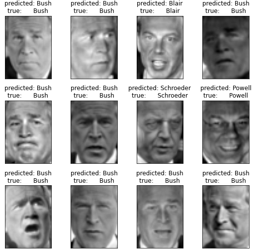
So, our accuracy is 0.85 and Results of our prediction are:
Reference:
Share your thoughts in the comments
Please Login to comment...