K Nearest Neighbors with Python | ML
Last Updated :
05 May, 2023
K-Nearest Neighbors is one of the most basic yet essential classification algorithms in Machine Learning. It belongs to the supervised learning domain and finds intense application in pattern recognition, data mining, and intrusion detection. The K-Nearest Neighbors (KNN) algorithm is a simple, easy-to-implement supervised machine learning algorithm that can be used to solve both classification and regression problems. The KNN algorithm assumes that similar things exist in close proximity. In other words, similar things are near to each other. KNN captures the idea of similarity (sometimes called distance, proximity, or closeness) with some mathematics we might have learned in our childhood— calculating the distance between points on a graph. There are other ways of calculating distance, which might be preferable depending on the problem we are solving. However, the straight-line distance (also called the Euclidean distance) is a popular and familiar choice. It is widely disposable in real-life scenarios since it is non-parametric, meaning, it does not make any underlying assumptions about the distribution of data (as opposed to other algorithms such as GMM, which assume a Gaussian distribution of the given data). This article illustrates K-nearest neighbors on a sample random data using sklearn library.
Importing Libraries and Dataset
Python libraries make it very easy for us to handle the data and perform typical and complex tasks with a single line of code.
- Pandas – This library helps to load the data frame in a 2D array format and has multiple functions to perform analysis tasks in one go.
- Numpy – Numpy arrays are very fast and can perform large computations in a very short time.
- Matplotlib/Seaborn – This library is used to draw visualizations.
- Sklearn – This module contains multiple libraries having pre-implemented functions to perform tasks from data preprocessing to model development and evaluation.
Python3
import pandas as pd
import seaborn as sns
import matplotlib.pyplot as plt
import numpy as np
|
Now let’s load the dataset using the pandas dataframe. You can download the dataset from here which has been used for illustration purpose in this article.
Python3
df = pd.read_csv("prostate.csv")
df.head()
|
Output:
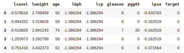
First Five rows of the dataset
Standardize the Variables
Because the KNN classifier predicts the class of a given test observation by identifying the observations that are nearest to it, the scale of the variables matters. Any variables that are on a large scale will have a much larger effect on the distance between the observations, and hence on the KNN classifier than variables that are on a small scale.
Python3
from sklearn.preprocessing import StandardScaler
scaler = StandardScaler()
scaler.fit(df.drop('Target', axis=1))
scaled_features = scaler.transform(df.drop('Target',
axis=1))
df_feat = pd.DataFrame(scaled_features,
columns=df.columns[:-1])
df_feat.head()
|
Output:
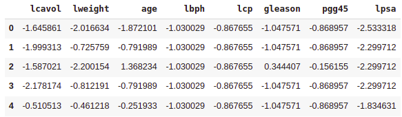
Features for the KNN model
Model Development and Evaluation
Now by using the sklearn library implementation of the KNN algorithm we will train a model on that. Also after the training purpose, we will evaluate our model by using the confusion matrix and classification report.
Python3
from sklearn.metrics import classification_report,\
confusion_matrix
from sklearn.neighbors import KNeighborsClassifier
from sklearn.model_selection import train_test_split
X_train, X_test,\
y_train, y_test = train_test_split(scaled_features,
df['Taregt'],
test_size=0.30)
knn = KNeighborsClassifier(n_neighbors=1)
knn.fit(X_train, y_train)
pred = knn.predict(X_test)
print(confusion_matrix(y_test, pred))
print(classification_report(y_test, pred))
|
Output:
[[19  3]
 [ 2  6]]
              precision    recall  f1-score   support

           0       0.90      0.86      0.88        22
           1       0.67      0.75      0.71         8

    accuracy                           0.83        30
   macro avg       0.79      0.81      0.79        30
weighted avg       0.84      0.83      0.84        30
Elbow Method
Let’s go ahead and use the elbow method to pick a good K Value.
Python3
error_rate = []
for i in range(1, 40):
knn = KNeighborsClassifier(n_neighbors=i)
knn.fit(X_train, y_train)
pred_i = knn.predict(X_test)
error_rate.append(np.mean(pred_i != y_test))
plt.figure(figsize=(10, 6))
plt.plot(range(1, 40), error_rate, color='blue',
linestyle='dashed', marker='o',
markerfacecolor='red', markersize=10)
plt.title('Error Rate vs. K Value')
plt.xlabel('K')
plt.ylabel('Error Rate')
plt.show()
|
Output:
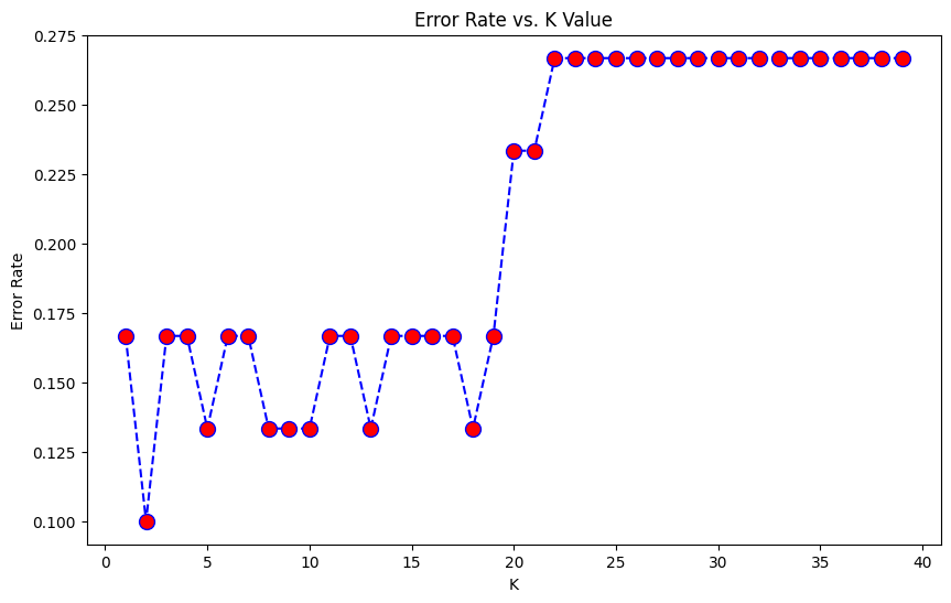
Elbow method to determine the number of clusters
Here we can observe that the error value is oscillating and then it increases to become saturated approximately. So, let’s take the value of K equal to 10 as that value of error is quite redundant.
Python3
knn = KNeighborsClassifier(n_neighbors = 1)
knn.fit(X_train, y_train)
pred = knn.predict(X_test)
print('WITH K = 1')
print('Confusion Matrix')
print(confusion_matrix(y_test, pred))
print('Classification Report')
print(classification_report(y_test, pred))
|
Output:
WITH K = 1
Confusion Matrix
[[19  3]
 [ 2  6]]
Classification Report
              precision    recall  f1-score   support

           0       0.90      0.86      0.88        22
           1       0.67      0.75      0.71         8

    accuracy                           0.83        30
   macro avg       0.79      0.81      0.79        30
weighted avg       0.84      0.83      0.84        30
Now let’s try to evaluate the performance of the model by using the number of clusters for which the error rate is the least.
R
knn = KNeighborsClassifier(n_neighbors = 10)
knn.fit(X_train, y_train)
pred = knn.predict(X_test)
print('WITH K = 10')
print('Confusion Matrix')
print(confusion_matrix(y_test, pred))
print('Classification Report')
print(classification_report(y_test, pred))
|
Output:
WITH K = 10
Confusion Matrix
[[21  1]
 [ 3  5]]
Classification Report
              precision    recall  f1-score   support

           0       0.88      0.95      0.91        22
           1       0.83      0.62      0.71         8

    accuracy                           0.87        30
   macro avg       0.85      0.79      0.81        30
weighted avg       0.86      0.87      0.86        30
Great! We squeezed some more performance out of our model by tuning it to a better K value.
Advantages of KNN:
- It is easy to understand and implement.
- It can also handle multiclass classification problems.
- Useful when data does not have a clear distribution.
- It works on a non-parametric approach.
Disadvantages of KNN:
- Sensitive to the noisy features in the dataset.
- Computationally expansive for the large dataset.
- It can be biased in the imbalanced dataset.
- Requires the choice of the appropriate value of K.
- Sometimes normalization may be required.
Share your thoughts in the comments
Please Login to comment...