Meta-analysis is a sophisticated statistical technique combining and analyzing data from multiple independent studies to obtain a more comprehensive and reliable estimate of the relationship or effect size between variables. It provides a means of systematically reviewing and synthesizing findings from individual studies to derive more robust conclusions.
The results obtained from the meta-analysis are interpreted and summarized, considering the overall effect size, confidence intervals, heterogeneity, and potential sources of bias. It is crucial to consider the context of the included studies and the limitations inherent in the meta-analysis.
Meta-analysis serves as an invaluable tool in evidence-based research and policy-making, as it allows researchers to synthesize data from multiple studies in a systematic manner. By integrating and analyzing a wide range of information, meta-analysis assists in identifying consistent patterns, detecting potential sources of variation, and providing more precise and reliable estimates of the relationship or effect size being investigated.
The steps involved in the meta-analysis are as follows:
- Define the research question: Clearly state the objective of the meta-analysis in machine learning, such as comparing the performance of different algorithms or evaluating the effectiveness of specific techniques.
- Search for relevant studies: Conduct a thorough search of the literature, including research papers and conference proceedings, to find studies or experiments that have explored similar research questions in machine learning.
- Select appropriate studies: Apply specific criteria to choose studies that meet the predetermined requirements, considering factors like study design, algorithms used, data characteristics, and relevance to the research question.
- Extract data: Gather relevant information from each selected study, such as details about the experimental setup, the dataset used, algorithm specifications, evaluation metrics, and performance results.
- Calculate effect size: Determine a suitable measure to compare the performance of machine learning models, such as accuracy or mean squared error. Compute the effect size for each study based on this measure.
- Analyze the data: Use statistical methods to combine the effect sizes from the selected studies, considering factors like study sample sizes. Compute summary statistics and perform hypothesis tests to assess the overall effect or differences between subgroups.
- Assess heterogeneity: Evaluate the variability among the effect sizes of the included studies using statistical tests and visual tools. Explore potential sources of variation, such as differences in datasets or model configurations, and conduct subgroup analyses if necessary.
- Evaluate publication bias: Investigate the possibility of publication bias, which occurs when studies with positive or statistically significant results are more likely to be published. Employ statistical tests, like funnel plots, to assess and account for any bias.
- Interpret and report the findings: Explain the results of the meta-analysis, considering the overall effect size, heterogeneity, and any identified patterns or subgroup differences. Provide a clear and accurate report, including limitations associated with the studies and the meta-analysis process in machine learning.
Features of meta-analysis:
- Integration of multiple studies: Meta-analysis involves a systematic collection and synthesis of data from various studies that have investigated the same or similar research question. This meticulous amalgamation of results from diverse studies enables a more robust and reliable estimation of the overall effect size.
- Statistical analysis: Meta-analysis utilizes sophisticated statistical methods to analyze the collected data from individual studies quantitatively. It transcends a mere narrative review by employing mathematical techniques to amalgamate the results and derive summary statistics.
- Effect size estimation: A primary objective of meta-analysis is to estimate the effect size of an intervention, treatment, or the relationship between variables. The effect size, a standardized measure, quantifies the magnitude and direction of the aforementioned relationship or the impact of a specific intervention.
- Heterogeneity assessment: Meta-analysis scrutinizes the heterogeneity or variability among the results of individual studies. This scrutiny entails evaluating disparities in study design, participant characteristics, interventions, or other factors that may contribute to the observed variability. Understanding heterogeneity is pivotal for interpreting the overall effect size and may necessitate subgroup analyses or further investigation.
- Publication bias assessment: Meta-analysis endeavors to identify and address publication bias, which denotes the inclination for studies with statistically significant results to be more likely published than those with non-significant or negative findings. Publication bias can distort the estimation of the overall effect size; therefore, it is crucial to assess and account for its potential impact.
- Forest plot: A forest plot, a widely-used graphical representation in the meta-analysis, exhibits the effect sizes and confidence intervals of individual studies, along with the summary effect size estimate. This visual representation facilitates the assessment of variability and the contribution of each study to the overall analysis.
- Subgroup analysis and meta-regression: Meta-analysis can explore potential sources of heterogeneity through subgroup analysis and meta-regression. Subgroup analysis stratifies the data based on specific characteristics (e.g., age, gender) to ascertain whether effect sizes differ across subgroups. Meta-regression investigates the relationship between study-level characteristics (e.g., sample size, study quality) and the effect sizes.
- Sensitivity analysis: Sensitivity analysis is conducted in meta-analysis to gauge the robustness of the results to various methodological choices or assumptions. By systematically varying certain parameters or excluding specific studies, researchers can examine the impact of such changes on the overall findings, thereby evaluating the stability and reliability of the results.
- Interpretation and reporting: Meta-analysis necessitates meticulous interpretation and reporting of the findings. Researchers should consider the limitations of the included studies, potential biases, and the implications of the results for the research question at hand. Transparent reporting guidelines, such as the Preferred Reporting Items for Systematic Reviews and Meta-Analyses (PRISMA), offer a framework for comprehensive reporting of meta-analytic studies.
Performing meta-analysis in R
To perform a meta-analysis in R, we can create a hypothetical dataset and then proceed with the meta-analysis using the “meta” package.
Install and load required packages.
In this step, we install the “meta” package using the install.packages() function. Once the package is installed, we load it into our R session using the library(meta) function. This makes the functions and capabilities of the “meta” package available for use.
R
install.packages("meta")
library(meta)
|
Create dataset
In this step, we generate hypothetical data for the meta-analysis. We set a seed using set. seed() to ensure the reproducibility of the random numbers generated. The variable n represents the number of studies.
We then use the rnorm() function to generate n random effect sizes from a normal distribution. The mean parameter is set to 0.5, and the sd parameter is set to 0.2. You can modify these values based on your specific scenario.
Next, we use the runif() function to generate n random variances. The min and max parameters control the range of random values. In this example, variances are randomly generated between 0.01 and 0.1. Adjust these values as needed.
R
set.seed(123)
n <- 100
effect_sizes <- rnorm(n, mean = 0.5, sd = 0.2)
variances <- runif(n, min = 0.01, max = 0.1)
|
Create a meta object.
In this step, we create a meta object to store the data for the meta-analysis. We first create a data frame called study_data that contains two columns: effect_size and variance. The effect_sizesizes column object sizes contain sizes containncemeta-object column sizes column function contains column sizes object column meta-object contains the corresponding variances for each study.
Next, we use the metagen() function to create the meta-objectthe. The metagen() the meta-object function takes several arguments:
TE: Specifies the column name (effect_size) in the study_data a meta-object column data frame that contains the treatment effect estimates (effect sizes) for each study.seTE: Specifies the column name (variance) in the study_data a data frame that contains the standard errors or variances corresponding to the treatment effect estimates.data: Specifies the data frame (study_data) that contains the meta-analysis data.
The metagen() function combines the treatment effect estimates and their corresponding variances to create the meta-object, which will be used for subsequent analysis and visualization.
R
study_data <- data.frame(effect_size = effect_sizes, variance = variances)
meta_object <- metagen(TE = effect_size, seTE = sqrt(variance), data = study_data)
|
Explore heterogeneity
In this step, we explore heterogeneity among the effect sizes using a forest plot. We use the forest() function from the “meta” package to generate the plot.
Heterogeneity in meta-analysis refers to the variability or differences in effect sizes observed across the included studies. It is an important consideration because it can influence the interpretation and generalizability of the meta-analysis results.
The forest plot is a graphical representation that helps visualize and assess heterogeneity among the effect sizes. It provides a visual summary of the individual study estimates, their precision (typically represented by confidence intervals), and the overall treatment effect estimate.
Output:
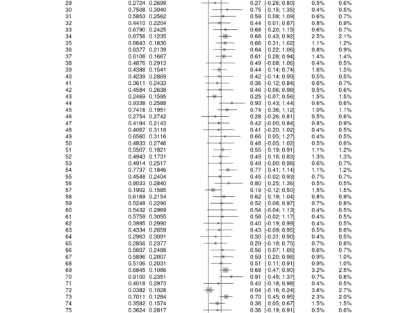
- Effect Sizes: In a meta-analysis, each study provides an estimate of the treatment effect, often represented as an effect size. Effect sizes quantify the magnitude and direction of the treatment effect observed in each study. Examples of effect size measures include mean differences, odds ratios, risk ratios, or hazard ratios.
- Confidence Intervals (CI): For each study, the effect size is accompanied by a confidence interval, which reflects the uncertainty associated with the effect size estimate. The confidence interval provides a range within which the true effect size is likely to fall. Wider confidence intervals indicate greater uncertainty, while narrower intervals indicate greater precision.
- Weighting: The forest plot uses weighting to give more or less emphasis to individual study estimates based on their precision. Studies with smaller standard errors (or larger sample sizes) are given more weight in the calculation of the overall treatment effect estimate.
- Overall Treatment Effect Estimate: The forest plot includes a summary estimate of the treatment effect, typically represented by a diamond-shaped marker or a solid vertical line. This summary estimate combines the individual study estimates, taking into account their weights based on precision.
- Horizontal Lines: Each study in the forest plot is represented by a horizontal line segment, known as a study marker. The position of the marker on the vertical axis represents the effect size estimate, and the horizontal line represents the confidence interval around the estimate.
- Vertical Line of No Effect: The forest plot usually includes a vertical line at the null or no-effect value (e.g., effect size = 0). This line helps to visualize whether the individual study estimates fall on either side of the null value.
- Heterogeneity Statistics: The forest plot may also include statistical measures of heterogeneity, such as Cochran’s Q statistic or the I-squared statistic. These measures quantify the degree of variability or inconsistency among the effect sizes across the studies. Higher values indicate greater heterogeneity.
By examining the forest plot, you can gain insights into the overall treatment effect estimate, the distribution of effect sizes across studies, the precision of the estimates, and the presence of heterogeneity. It helps identify studies with large or influential effect sizes, explore the consistency of results, and detect potential sources of heterogeneity.
Conduct statistical analysis
In this step, we conduct a statistical analysis of the meta-analysis results using the summary() function from the “meta” package.
By using the summary() function, you can gain valuable insights into the meta-analysis results. It allows you to determine the overall treatment effect and its significance, assess the precision of the estimate, evaluate the presence and extent of heterogeneity, and obtain a summary of the forest plot findings. These insights aid in drawing meaningful conclusions and informing decision-making regarding the treatment’s effectiveness in the meta-analysis.
Useful results summary() function provides:
- Overall Treatment Effect Estimate: The
summary() the function provides an estimate of the overall treatment effect based on the combined evidence from all the included studies.
- Confidence Intervals: Along with the overall treatment effect estimate, the
summary() function calculates the confidence interval (CI) around the estimate. The CI provides a range within which the true effect size is likely to fall with a certain level of confidence.
- Heterogeneity Statistics: The
summary() the function also reports statistical measures of heterogeneity. One commonly used measure is I-squared (I²), which represents the proportion of total variation in effect sizes that can be attributed to heterogeneity rather than chance.
- Forest Plot Recap: The
summary() the function provides a summary of the forest plot generated in Step 4. It repeats the overall treatment effect estimate, confidence intervals, and heterogeneity statistics.
- Test of Overall Treatment Effect: The
summary() the function performs a statistical test to evaluate whether the overall treatment effect estimate is statistically significant. The test typically involves comparing the estimated treatment effect to the null hypothesis of no effect (e.g., effect size = 0).
- Sensitivity Analysis: The
summary() a function may also offer options for conducting sensitivity analyses. These analyses assess the robustness of the meta-analysis results to different assumptions or variations in the inclusion criteria, statistical methods, or study characteristics.
Assess publication bias
In this step, we assess publication bias using a funnel plot. We use the funnel() function from the “meta” package to generate the plot.
Publication bias refers to the phenomenon where published studies are systematically biased towards reporting statistically significant or positive results, while studies with non-significant or negative results are less likely to be published. Assessing publication bias is important in meta-analysis as it can impact the validity and generalizability of the findings.
Output:
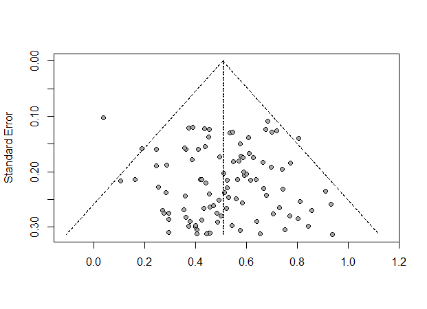
A funnel plot is a graphical tool used to assess publication bias visually. It helps examine the relationship between the effect sizes (or treatment estimates) and their precision (typically represented by the standard errors or sample sizes) across the included studies. We can derive the following results from a funnel chart:
- Effect Sizes: The effect sizes represent the treatment estimates observed in each study.
- Precision Measures: The precision measures represent the level of uncertainty associated with the effect sizes.
- Funnel Shape: In the absence of publication bias, the funnel plot exhibits a symmetrical inverted funnel shape.
- Publication Bias: Publication bias can be observed as an asymmetry in the funnel plot. If publication bias is present, smaller studies with non-significant or negative results may be missing from the plot, leading to a “missing” region on one side of the funnel.
- Assessing Publication Bias: The funnel plot is visually inspected to assess publication bias. Deviations from symmetry can indicate the presence of publication bias.
- Statistical Tests: Various statistical tests can be conducted to formally assess publication bias. Some commonly used tests include Egger’s test, Begg’s test, and the trim-and-fill method. These tests examine the relationship between the effect sizes and their precision and provide statistical evidence of publication bias.
By examining the funnel plot and conducting statistical tests, you can gain insights into the presence and extent of publication bias in the meta-analysis. These insights help evaluate the potential impact of publication bias on the overall findings and interpretation of the meta-analysis results.
In this way, we have finally done a meta-analysis in R and understood its important steps.
Meta-analysis in R on a custom dataset
Here’s a step-by-step explanation of the code for performing a basic meta-analysis using custom data in R:
Create the Data
- We start by creating a data frame named
custom_data that represents our custom dataset.
- The
custom_data data frame includes columns such as study_id, effect_size, and variance.
- Each row in the data frame corresponds to a different study, with the
effect_size representing the effect size estimate and variance representing the variance or standard error of the effect size estimate.
R
custom_data <- data.frame(
study_id = c("Study 1", "Study 2", "Study 3"),
effect_size = c(0.5, 0.8, 1.2),
variance = c(0.1, 0.15, 0.2)
)
|
Load the Necessary Packages
- We load the
meta package, which provides functions for conducting meta-analyses in R.
- The
meta package contains various functions that facilitate the meta-analysis process.
Create the Meta-analysis Object
- We create the meta-analysis object named
meta_object using the metagen() function from the meta package.
- The
metagen() the function is used for conducting meta-analyses of continuous outcomes.
- Inside the
metagen() function, we specify the necessary arguments:
TE: We provide the effect sizes from the custom_data$effect_size column.seTE: We provide the standard errors calculated as the square root of the variances from the custom_data$variance column.data: We specify the custom_data data frame as the source of the data.
R
meta_object <- metagen(
TE = custom_data$effect_size,
seTE = sqrt(custom_data$variance),
data = custom_data
)
|
Visualize Heterogeneity using a Forest Plot
- We use the
forest() function from the meta package to create a forest plot, which visualizes the effect sizes of individual studies along with their confidence intervals.
- The
forest() function takes the meta_object as an input.
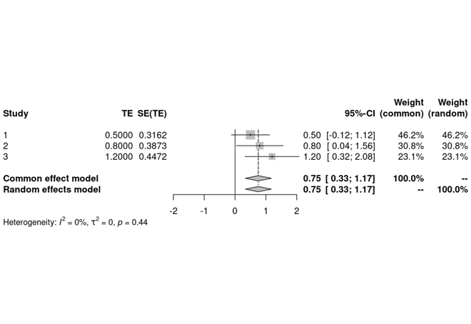
Forest Plot for custom data
Obtain a Summary of the Meta-analysis Results
- We use the
summary() function from the meta package to obtain a summary of the meta-analysis results.
- The
summary() the function provides information such as the overall effect size estimate, confidence intervals, and statistical measures of heterogeneity.
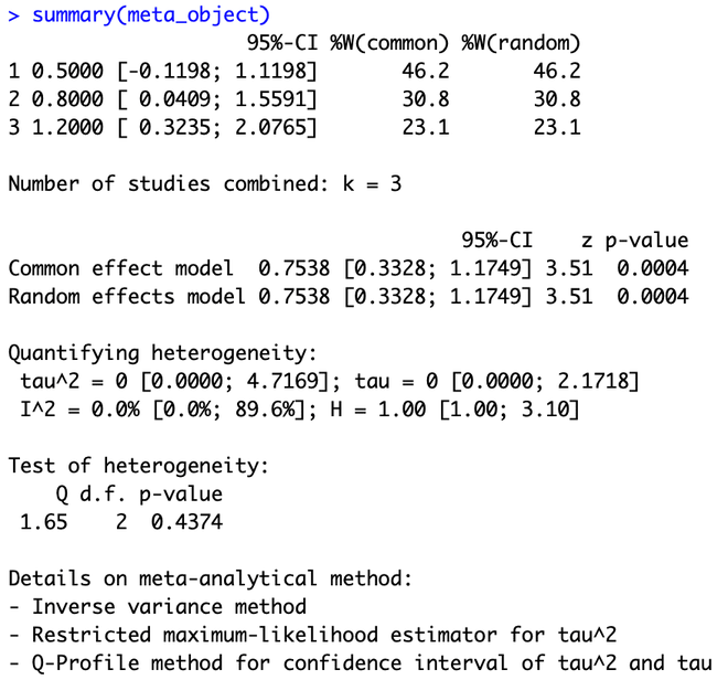
Summary of meta analysis
Assess Publication Bias using a Funnel Plot
- We use the
funnel() function from the meta package to create a funnel plot, which helps assess publication bias.
- The funnel plot examines the relationship between the effect sizes and their corresponding standard errors.
- The
funnel() function takes the meta_object as an input.
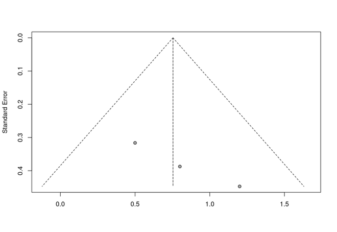
Funnel Chart
These steps together allow you to conduct a basic meta-analysis using custom data in R.
Share your thoughts in the comments
Please Login to comment...