How to Perform Hierarchical Cluster Analysis using R Programming?

Cluster analysis or clustering is a technique to find subgroups of data points within a data set. The data points belonging to the same subgroup have similar features or properties. Clustering is an unsupervised machine learning approach and has a wide variety of applications such as market research, pattern recognition, recommendation systems, and so on. The most common algorithms used for clustering are K-means clustering and Hierarchical cluster analysis. In this article, we will learn about hierarchical cluster analysis and its implementation in R programming.

Hierarchical cluster analysis (also known as hierarchical clustering) is a clustering technique where clusters have a hierarchy or a predetermined order. Hierarchical clustering can be represented by a tree-like structure called a Dendrogram. There are two types of hierarchical clustering:

• Agglomerative hierarchical clustering: This is a bottom-up approach where each data point starts in its own cluster and as one moves up the hierarchy, similar pairs of clusters are merged.
• Divisive hierarchical clustering: This is a top-down approach where all data points start in one cluster and as one moves down the hierarchy, clusters are split recursively.

To measure the similarity or dissimilarity between a pair of data points, we use distance measures (Euclidean distance, Manhattan distance, etc.). However, to find the dissimilarity between two clusters of observations, we use agglomeration methods. The most common agglomeration methods are:

• Complete linkage clustering: It computes all pairwise dissimilarities between the observations in two clusters, and considers the longest (maximum) distance between two points as the distance between two clusters.
• Single linkage clustering: It computes all pairwise dissimilarities between the observations in two clusters, and considers the shortest (minimum) distance as the distance between two clusters.
• Average linkage clustering: It computes all pairwise dissimilarities between the observations in two clusters, and considers the average distance as the distance between two clusters.

Performing Hierarchical Cluster Analysis using R

For computing hierarchical clustering in R, the commonly used functions are as follows:

• hclust in the stats package and agnes in the cluster package for agglomerative hierarchical clustering.
• diana in the cluster package for divisive hierarchical clustering.

We will use the Iris flower data set from the datasets package in our implementation. We will use sepal width, sepal length, petal width, and petal length column as our data points. First, we load and normalize the data. Then the dissimilarity values are computed with dist function and these values are fed to clustering functions for performing hierarchical clustering. 

R

# Load required packages
library(datasets) # contains iris dataset
library(cluster)  # clustering algorithms
library(factoextra) # visualization
library(purrr) # to use map_dbl() function

# Load and preprocess the dataset
df <- iris[, 1:4]
df <- na.omit(df)
df <- scale(df)

# Dissimilarity matrix
d <- dist(df, method = "euclidean")

Agglomerative hierarchical clustering implementation

The dissimilarity matrix obtained is fed to hclust. The method parameter of hclust specifies the agglomeration method to be used (i.e. complete, average, single). We can then plot the dendrogram.

R

# Hierarchical clustering using Complete Linkage
hc1 <- hclust(d, method = "complete" )

# Plot the obtained dendrogram
plot(hc1, cex = 0.6, hang = -1)

Output:

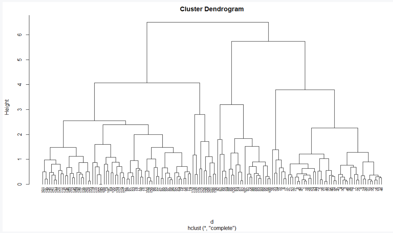
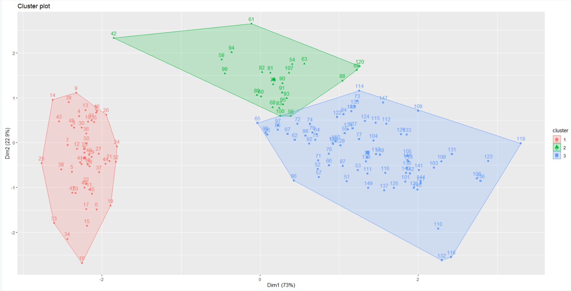
Observe that in the above dendrogram, a leaf corresponds to one observation and as we move up the tree, similar observations are fused at a higher height. The height of the dendrogram determines the clusters. In order to identify the clusters, we can cut the dendrogram with cutree. Then visualize the result in a scatter plot using fviz_cluster function from the factoextra package.

R

# Cut tree into 3 groups
sub_grps <- cutree(hc1, k = 3)

# Visualize the result in a scatter plot
fviz_cluster(list(data = df, cluster = sub_grps))

Output:

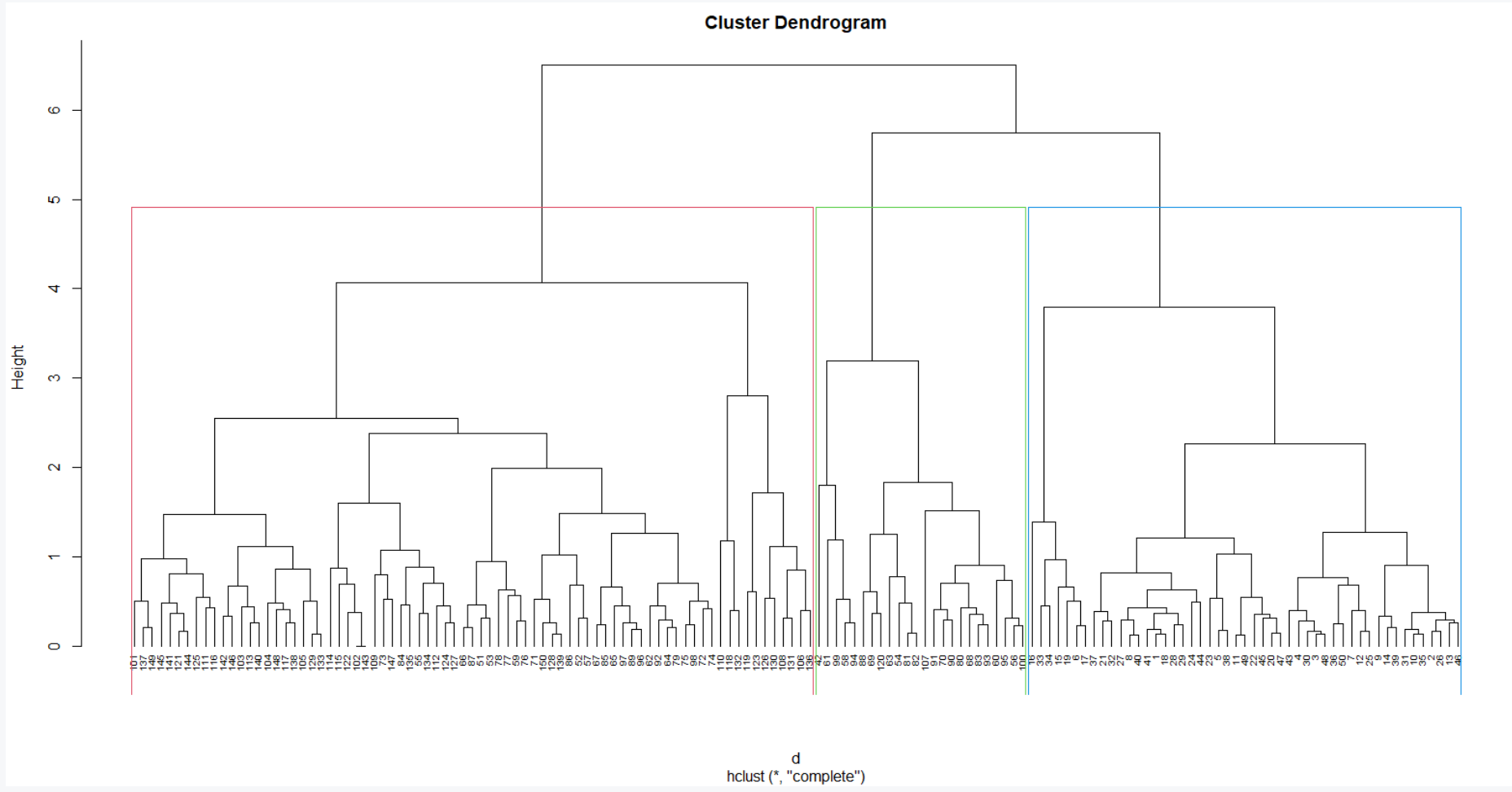
We can also provide a border to the dendrogram around the 3 clusters as shown below.

R

# Plot the obtained dendrogram with
# rectangle borders for k clusters
plot(hc1, cex = 0.6, hang = -1)
rect.hclust(hc1, k = 3, border = 2:4)

Output:

Alternatively, we can use the agnes function to perform the hierarchical clustering. Unlike hclust, the agnes function gives the agglomerative coefficient, which measures the amount of clustering structure found (values closer to 1 suggest strong clustering structure).

R

# agglomeration methods to assess
m <- c("average", "single", "complete")
names(m) <- c("average", "single", "complete")

# function to compute hierarchical
# clustering coefficient
ac <- function(x) {
  agnes(df, method = x)$ac
}

map_dbl(m, ac)

Output:

 average    single  complete 
0.9035705 0.8023794 0.9438858 

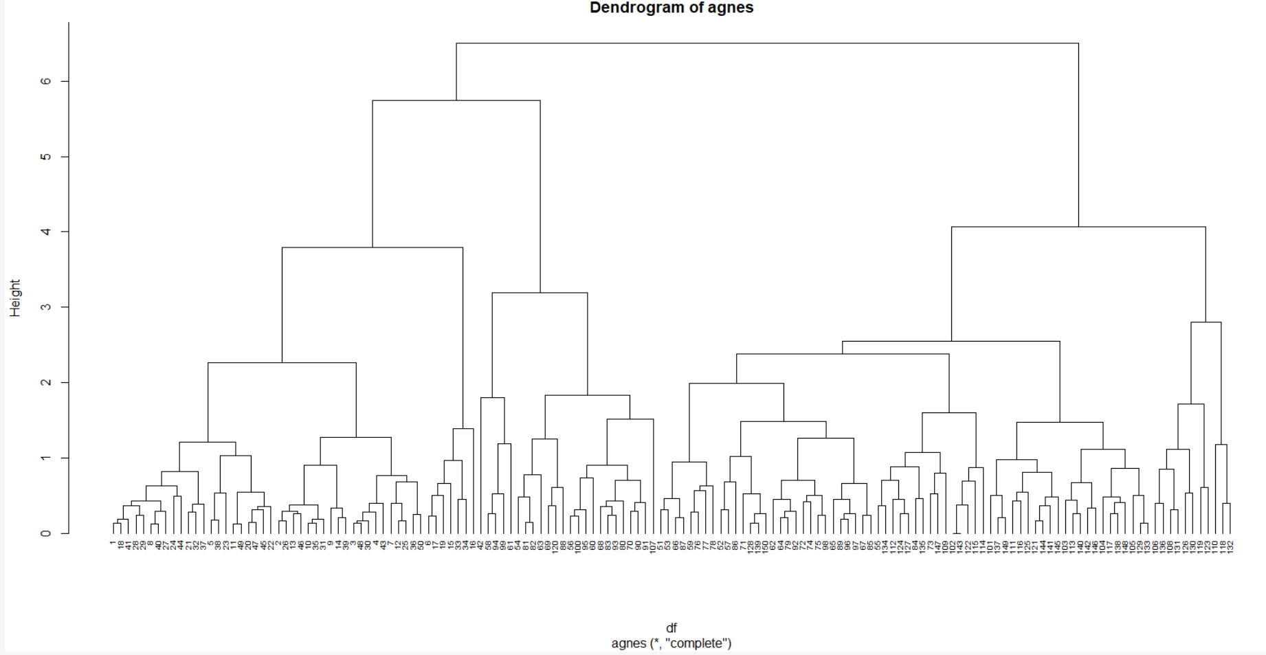
Complete linkage gives a stronger clustering structure. So, we use this agglomeration method to perform hierarchical clustering with agnes function as shown below.

R

# Hierarchical clustering
hc2 <- agnes(df, method = "complete")

# Plot the obtained dendrogram
pltree(hc2, cex = 0.6, hang = -1,
       main = "Dendrogram of agnes")

Output:

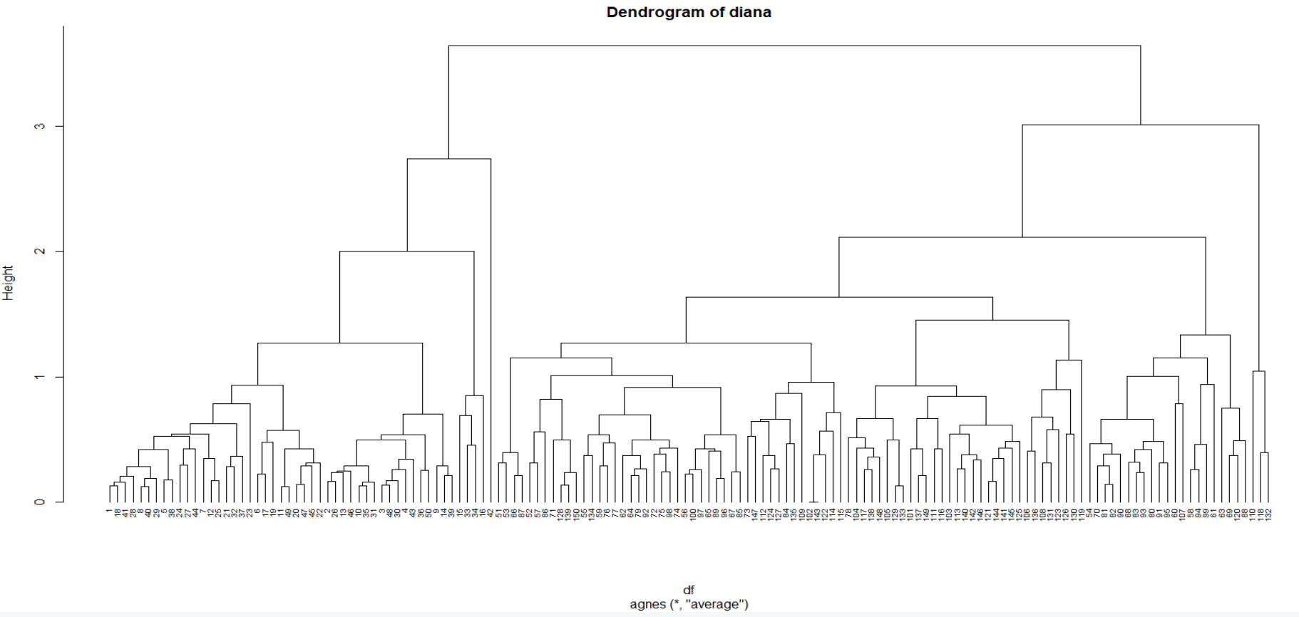
Divisive clustering implementation

The function diana which works similar to agnes allows us to perform divisive hierarchical clustering. However, there is no method to provide.

R

# Compute divisive hierarchical clustering
hc3 <- diana(df)

# Divise coefficient
hc3$dc

# Plot obtained dendrogram
pltree(hc3, cex = 0.6, hang = -1,
       main = "Dendrogram of diana")

Output:

[1] 0.9397208