How To Make Scree Plot in R with ggplot2

In this article, we are going to see how can we plot a Scree plot in R Programming Language with ggplot2. 

Loading dataset:

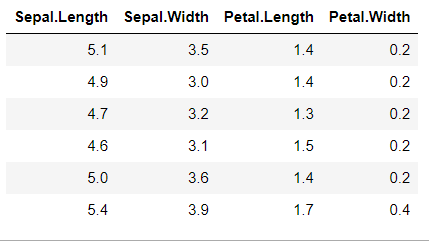
Here we will load the dataset, (Remember to drop the non-numerical column). Since the iris flower dataset contains a species column that is of character type so we need to drop it because PCA works with only numerical data.

R

# drop the species column as its character type
num_iris = subset(iris,
                  select = -c(Species))
head(num_iris)

Output:

Compute Principal Component Analysis using prcomp() function

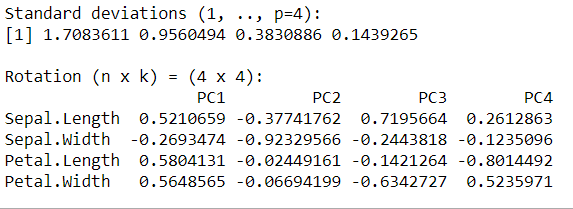
We use R language’s inbuilt prcomp() function, this function takes the dataset as an argument and computes the PCA. Principal Component Analysis (PCA) is a statistical procedure that uses an orthogonal transformation that converts a set of correlated variables to a set of uncorrelated variables. Doing scale=TRUE standardizes the data. 

Syntax: prcomp(numeric_data, scale = TRUE)

Code:

R

# drop the species column as its character type
num_iris = subset(iris, select = -c(Species) )

# compute pca
pca <- prcomp(num_iris, scale = TRUE)
pca

Output:

Compute variance explained by each Principal Component:

We use the formula below to compute the total variance experienced by each PC. 

Syntax: pca$sdev^2 / sum(pca$sdev^2)

Code:

R

# drop the species column as its character type
num_iris = subset(iris, select = -c(Species) )

# compute pca
pca <- prcomp(num_iris, scale = TRUE)

# compute total variance
variance = pca$sdev^2 / sum(pca$sdev^2)
variance

Output:

[1] 0.729624454 0.228507618 0.036689219 0.005178709

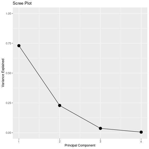
Example 1: Plotting Scree plot with Line plot

R

library(ggplot2)

# drop the species column as its character type
num_iris = subset(iris, select = -c(Species) )

# compute pca
pca <- prcomp(num_iris, scale = TRUE)

# compute total variance
variance = pca $sdev^2 / sum(pca $sdev^2)

# Scree plot
qplot(c(1:4), variance) +
  geom_line() +
  geom_point(size=4)+
  xlab("Principal Component") +
  ylab("Variance Explained") +
  ggtitle("Scree Plot") +
  ylim(0, 1)

Output:

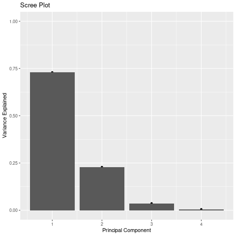
Example2: Plotting Scree plot with barplot

R

library(ggplot2)

# drop the species column as its character type
num_iris = subset(iris, select = -c(Species) )

# compute pca
pca <- prcomp(num_iris, scale = TRUE)

# compute total variance
variance = pca $sdev^2 / sum(pca $sdev^2)

# Scree plot
qplot(c(1:4), variance) +
  geom_col()+
  xlab("Principal Component") +
  ylab("Variance Explained") +
  ggtitle("Scree Plot") +
  ylim(0, 1)

Output: