How to Create a Digital Planner in Google Sheets

Welcome to the world of high-tech planning! Today, we’re diving into the fun of making your own Digital Planner using Google Sheets. Say goodbye to paper mess and hello to a stylish and super-organized way of managing your schedule and goals.

No worries if you’re new to digital planning – we’ve got your back! We’ll guide you through using Google Sheets, so you can customize your planner with ease. Get ready to kick the old-fashioned planners to the curb and step into the future of planning with our simple tips and tricks. Let’s create your Digital Planner and make organizing a breeze!

Create a Digital Planner in Google Sheets

To plan our year ahead a functional dynamic calendar planner with interactive UI is a must. With the help of Google Sheets, we can easily have one. So here are the steps to do that.

Working on Google Sheets can be confusing sometimes as it offers a lot of shortcuts and formulas, so try to follow my tutorial and do the same, and then you can play around and make a dynamic calendar that matches your aesthetic.

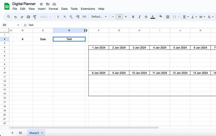
Step 1: Creating the calendar area (Week wise)

• Select a cell (here I have selected F4) and click on Data > Data Validation > Add rule.

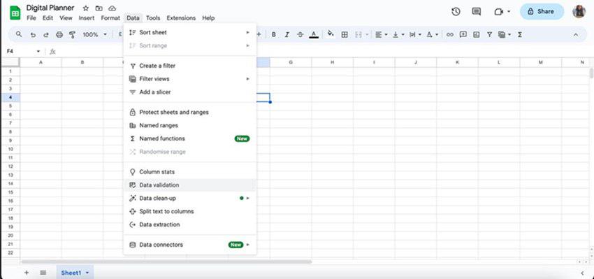
• In Add Rule, go to the criteria drop-down and select ‘Is valid date’ then select Reject the Input and click on ‘Done’. This will give your cell (F4) a calendar drop-down every time you click on it.

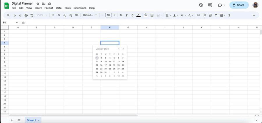
• Select a date of your choice for F4 from the drop-down calendar.

• Now, to get 7 consecutive days, select the cell next to F4 and apply the formula ‘=F4+1’ and enter. This will give you the next date.

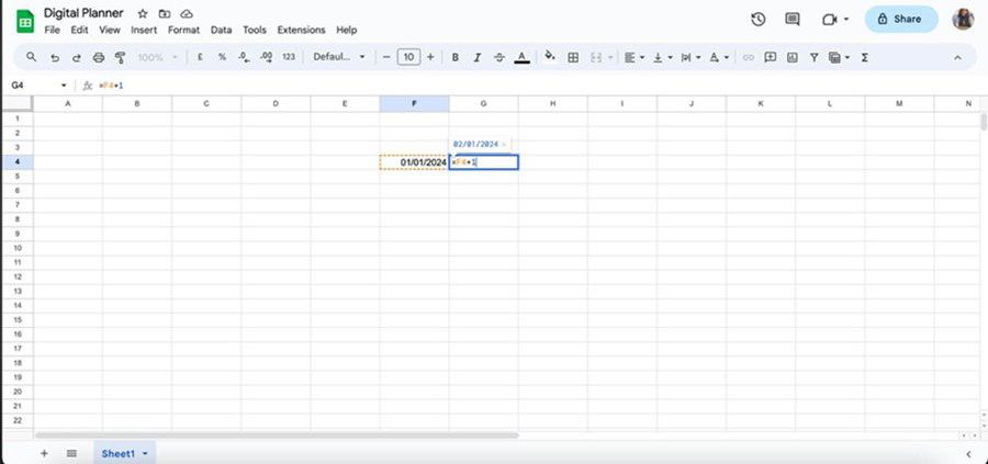
• Repeat this to get 7 consecutive days (as we are making week week-wise calendar).
• Leave 6 rows below your dated column (to add tasks) and add more dates (as shown in the pictures below).

Step 2: Customising the calendar area

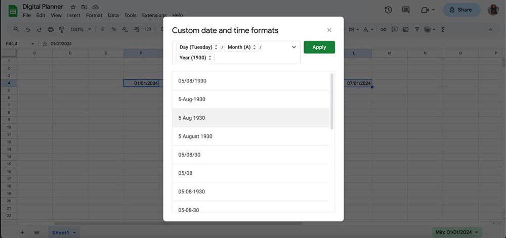
• To change the way the dates look, go to format > Number > Custom Date and Time.

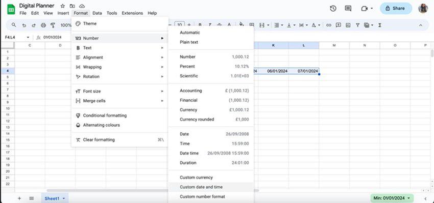
• Now from Custom date and time select the way you want your date to look.

• Also, to change the alignment to centre, select the whole table from the corner and change the alignment to centre.
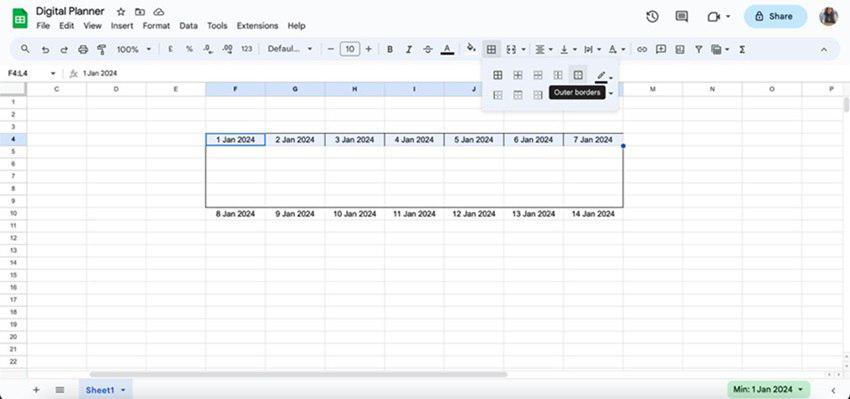
• You can also add borders to the dates and the space below them by selecting the dated rows and clicking on the border ( as shown in the picture).

Step 3: Adding a row for days

This will increase the functionality of our calendar as it will show the days above the dates.

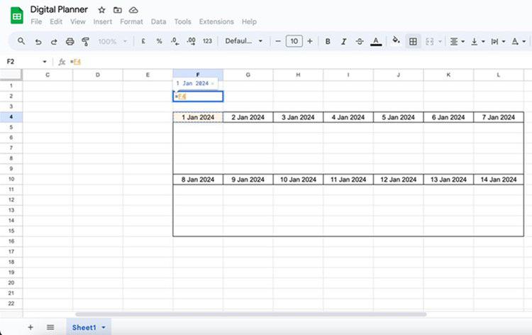
• Select the F2 column write ‘=F4’ and press ENTER. You will get the same date as F4.

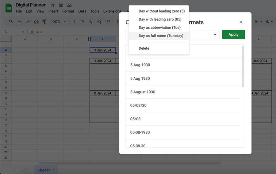
• Now select the whole row of F2 and go to Format > Number > Custom Date and Time.

• From Custom date and time select the option to show only the day.

• Drag the next 7 rows to get the same dates as the F4 rows (refer to the picture for a better understanding).

Step 4: Creating the task area

• Select column A, press ctrl (command for Mac users) select column E then decrease the width as per your choice.

• Then add labels to columns A, B and C as S.no./#, Date and task respectively.

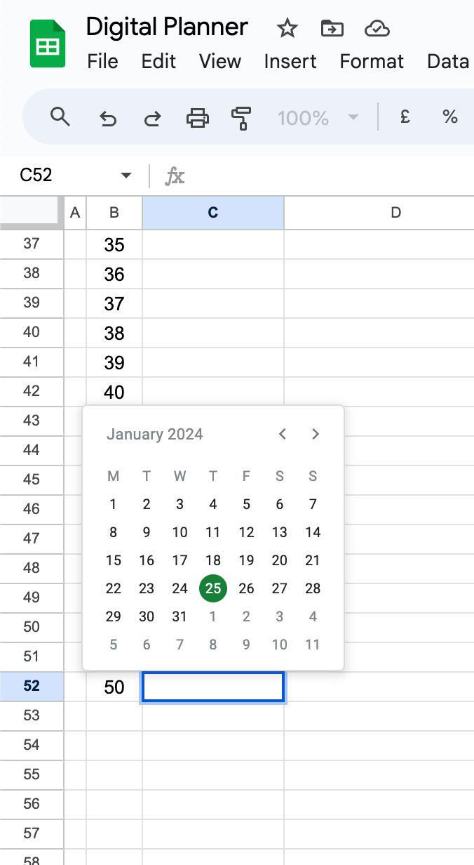
• For column B i.e. Serial number column, in order to add numbers we can write the formula ‘=sequence(50,1,1,1)’ and this would give us a sequence of 1-50 numbers. You can add more numbers to it as per your need.

Entering the formula

The result after the formula

• For column C i.e. the date column, repeat the same steps to add a drop-down calendar and convert it to the same format as the calendar area.

• For column D i.e. the task area, we want to create it in such a way that when we write a task for a respective day it should be displayed in the calendar area. This can be done by:
• Go to F5 cell and write ‘=FILTER(D4:D53, C4:C53 = F4)’. This will put a filter to our calendar area stating that range D4:D53 (range of task) will be displayed here if the condition C4:C53 (means from cell C4 to cell C53) is equal to the date/font of F4.
• Repeat the same for all the other dates by changing the RHS after equal to the current date cell ( as shown in the picture).

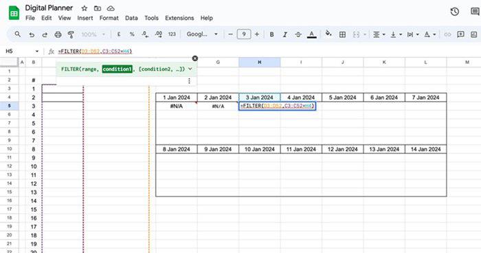
• In case there is no task for a particular date, N/A will be printed.
• Now, if you put a date and a task next to that and hit ENTER in the task area, it will automatically appear in the calendar area.

Step 5: Customising the dynamic calendar

• Select the task area column and add borders of your choice.
• Add colours to your calendar to make it look more attractive.

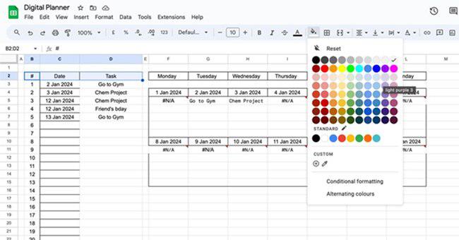
• You can add more dates as per your requirement and basically play around.
• The lines in the spreadsheet can also be removed by clicking on View > gridline.

Step 6: Preview Results

Final Result

FAQs

Can we add more rows in the calendar area?

Yes, more rows can be added by selecting a cell from the left and right click then select ‘insert 1 row’.

How are borders added?

Select the area you want to give a border then find the border icon (right next to the paint icon) above and select the desired type of border for your area. There are many options to choose from.

Is it possible to print something else in place of N/A for a date with no task?

Yes, it is possible. It can be done by adding this formula ‘ IFERROR(FILTER(D4:D53, C4:C53=F4), No Event)’. You can add any text in place of ‘No Event’ or keep it empty.

How to add more weeks to the dynamic calendar?

Copy the week above (including the space for task) and paste it below. Repeat it get the desired number of weeks.

Whether you’re preparing for your first job interview or aiming to upskill in this ever-evolving tech landscape, GeeksforGeeks Courses are your key to success. We provide top-quality content at affordable prices, all geared towards accelerating your growth in a time-bound manner. Join the millions we’ve already empowered, and we’re here to do the same for you. Don’t miss out – check it out now!