Regression using CatBoost

In this article, we will learn about one of the state-of-the-art machine learning models: Catboost here cat stands for categorical which implies that this algorithm is highly efficient when your data contains many categorical columns.

What is CatBoost?

CatBoost, (Categorical Boosting), is a high-performance, open-source, gradient-boosting framework developed by Yandex. It is designed for solving a wide range of machine learning tasks, including classification, regression, and ranking, with a particular emphasis on handling categorical features efficiently. Catboost stands out for its speed, accuracy, and ease of use in dealing with structured data.

How Catboost Works?

Catboost is a high-performance gradient-boosting technique made for machine learning tasks, especially in situations involving structured input. Gradient boosting, an ensemble learning technique, forms the basis of its main workings. Catboost begins by speculating, frequently the mean of the target variable. The ensemble of decision trees is then gradually built, with each tree seeking to eliminate the errors or residuals from the previous ones. Catboost stands out because of how well it handles category features. Catboost uses a method termed “ordered boosting” to process categorical data directly, resulting in faster training and better model performance.

Additionally, regularization techniques are incorporated to avoid overfitting. Catboost integrates the predictions from all the trees when making predictions, creating models that are extremely accurate and reliable. Additionally, it offers feature relevance rankings that help with feature selection and comprehension of model choices. Catboost is a useful tool for a variety of machine-learning tasks, such as classification, regressions, etc.

Implementation of Regression Using CatBoost

We will use this dataset to perform a regression task using the catboost algorithm. But to use the catboost model we will first have to install the catboost package model using the below command:

Installing Packages

!pip install catboost

Importing Libraries and Dataset

Python libraries make it very easy for us to handle the data and perform typical and complex tasks with a single line of code.

• Pandas – This library helps to load the data frame in a 2D array format and has multiple functions to perform analysis tasks in one go.
• Numpy – Numpy arrays are very fast and can perform large computations in a very short time.
• Matplotlib/Seaborn – This library is used to draw visualizations.
• Sklearn – This module contains multiple libraries having pre-implemented functions to perform tasks from data preprocessing to model development and evaluation.

Python3

#importing libraries
import pandas as pd
import numpy as np
import seaborn as sb
import matplotlib.pyplot as plt
import lightgbm as lgb

from sklearn.preprocessing import StandardScaler
from sklearn.model_selection import train_test_split

import warnings
warnings.filterwarnings('ignore')

Loading Dataset and Retriving Information

Python3

#loading dataset
df = pd.read_csv('House_Rent_Dataset.csv')
print(df.head())

Output:

    Posted On  BHK   Rent  Size            Floor    Area Type  \
0  2022-05-18    2  10000  1100  Ground out of 2   Super Area   
1  2022-05-13    2  20000   800       1 out of 3   Super Area   
2  2022-05-16    2  17000  1000       1 out of 3   Super Area   
3  2022-07-04    2  10000   800       1 out of 2   Super Area   
4  2022-05-09    2   7500   850       1 out of 2  Carpet Area   
              Area Locality     City Furnishing Status  Tenant Preferred  \
0                    Bandel  Kolkata       Unfurnished  Bachelors/Family   
1  Phool Bagan, Kankurgachi  Kolkata    Semi-Furnished  Bachelors/Family   
2   Salt Lake City Sector 2  Kolkata    Semi-Furnished  Bachelors/Family   
3               Dumdum Park  Kolkata       Unfurnished  Bachelors/Family   
4             South Dum Dum  Kolkata       Unfurnished         Bachelors   
   Bathroom Point of Contact  
0         2    Contact Owner  
1         1    Contact Owner  
2         1    Contact Owner  
3         1    Contact Owner  
4         1    Contact Owner  

Here, we are loading the dataset and printing the top five rows in the datset.

Python3

#printing the shape of the dataset
df.shape

Output:

(4746, 12)

Here, ‘df.shape’ prints the dimensions of the dataframe ‘df’.

Python3

# Display summary information about the DataFrame 'df'
df.info()

Output:

<class 'pandas.core.frame.DataFrame'>
RangeIndex: 4746 entries, 0 to 4745
Data columns (total 12 columns):
 #   Column             Non-Null Count  Dtype 
---  ------             --------------  ----- 
 0   Posted On          4746 non-null   object
 1   BHK                4746 non-null   int64 
 2   Rent               4746 non-null   int64 
 3   Size               4746 non-null   int64 
 4   Floor              4746 non-null   object
 5   Area Type          4746 non-null   object
 6   Area Locality      4746 non-null   object
 7   City               4746 non-null   object
 8   Furnishing Status  4746 non-null   object
 9   Tenant Preferred   4746 non-null   object
 10  Bathroom           4746 non-null   int64 
 11  Point of Contact   4746 non-null   object
dtypes: int64(4), object(8)
memory usage: 445.1+ KB

Here, ‘df.info()’ displays the summary information about the dataframe ‘df’. It provides details such as no. of null-entries in each column, data types, and memory usage.

Python3

# Generate summary statistics of the DataFrame 'df'
print(df.describe())

Output:

               BHK          Rent         Size     Bathroom
count  4746.000000  4.746000e+03  4746.000000  4746.000000
mean      2.083860  3.499345e+04   967.490729     1.965866
std       0.832256  7.810641e+04   634.202328     0.884532
min       1.000000  1.200000e+03    10.000000     1.000000
25%       2.000000  1.000000e+04   550.000000     1.000000
50%       2.000000  1.600000e+04   850.000000     2.000000
75%       3.000000  3.300000e+04  1200.000000     2.000000
max       6.000000  3.500000e+06  8000.000000    10.000000

Here, ‘df.describe()’ computes and displays basic statistical summary information for the numeric columns in the dataframe.

Exploratory Data Analysis

EDA is an approach to analyzing the data using visual techniques. It is used to discover trends, and patterns, or to check assumptions with the help of statistical summaries and graphical representations. While performing the EDA of this dataset we will try to look at what is the relation between the independent features that is how one affects the other.

Python3

# Identify and collect categorical columns with less than 10 unique values
# Initialize an empty list to store categorical columns
cat_cols = []

# Iterate through DataFrame columns
for col in df.columns:
    if df[col].dtype == 'object' and df[col].nunique() < 10:
        # Add the column to the list
        cat_cols.append(col)
cat_cols += ['BHK', 'Bathroom']
cat_cols

Output:

['Area Type',
 'City',
 'Furnishing Status',
 'Tenant Preferred',
 'Point of Contact',
 'BHK',
 'Bathroom']

Categorical Count Plots

Now let’s observe the distribution of the whole data into these categorical columns categories by using a countplot from seaborn.

Python3

# Create subplots to display count plots for categorical columns in 'cat_cols'
# Subplots are arranged in a 4x2 grid, and
# each subplot shows the count distribution of a categorical column.
plt.subplots(figsize=(15, 15))
for i, col in enumerate(cat_cols):
    plt.subplot(4, 2, i+1)
    sb.countplot(data=df, x=col)
# Ensures proper spacing between subplots
plt.tight_layout()
# Display the subplots
plt.show()

Output:

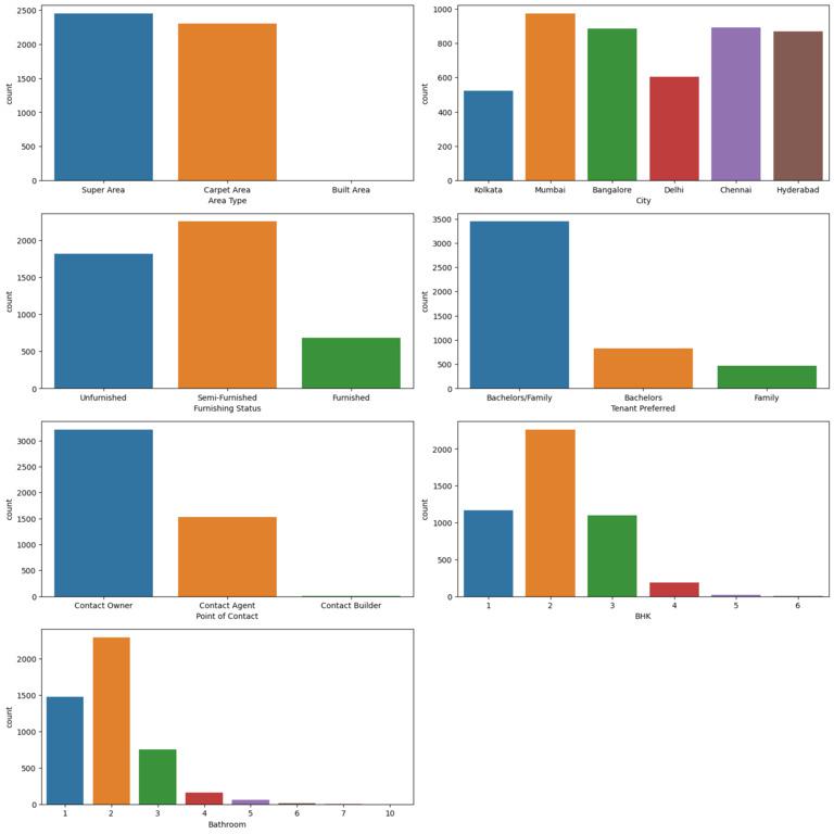
Here, each plot displays the distribution of counts for a specific categorical column. The ‘plt.tight_layout’ function ensures that the subplots are properly spaced, and ‘plt_show’ displays the grid of the count plots.

Numeric Distribution Plots

To understand the numerical data and its distribution density plots are considered as one of the best tools.

Python3

# Create subplots to display distribution plots for numeric columns in 'num_cols'
num_cols = ['Rent', 'Size']
plt.subplots(figsize=(10, 5))
for i, col in enumerate(num_cols):
    plt.subplot(1, 2, i+1)
    sb.distplot(df[col])
plt.tight_layout()
plt.show()

Output:

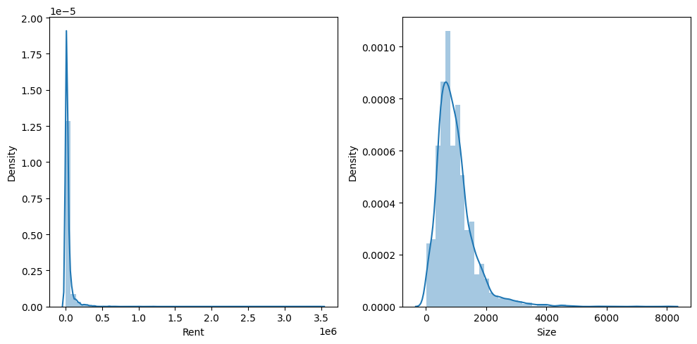
Here we can observe that the both rent and the size column are not normally distributed and it is considered as best practices to have the target and the features columns normally distributed for better results while using regressions in machine learning. To achieve this one of the famous method is logarithmic transformation that we will do in this article later before feeding the data to the model.

Python3

# Remove unnecessary columns
# ('Posted On', 'Floor', 'Area Locality') from the DataFrame 'df'
df.drop(['Posted On', 'Floor', 'Area Locality'],
        inplace=True, axis=1)

# For each categorical column in 'cat_cols',
# calculate and print the mean rent for each category
for i, col in enumerate(cat_cols):
    print(df[[col, 'Rent']].groupby(col).mean())
    print()

Output:

                     Rent
Area Type                
Built Area   10500.000000
Carpet Area  52385.897302
Super Area   18673.396566
                   Rent
City                   
Bangalore  24966.365688
Chennai    21614.092031
Delhi      29461.983471
Hyderabad  20555.048387
Kolkata    11645.173664
Mumbai     85321.204733
                           Rent
Furnishing Status              
Furnished          56110.305882
Semi-Furnished     38718.810751
Unfurnished        22461.635813
                          Rent
Tenant Preferred              
Bachelors         42143.793976
Bachelors/Family  31210.792683
Family            50020.341102
                          Rent
Point of Contact              
Contact Agent     73481.158927
Contact Builder    5500.000000
Contact Owner     16704.206468
              Rent
BHK               
1     14139.223650
2     22113.864018
3     55863.062842
4    168864.555556
5    297500.000000
6     73125.000000
                   Rent
Bathroom               
1          11862.162144
2          25043.538193
3          63176.698264
4         167846.153846
5         252350.000000
6         177500.000000
7          81666.666667
10        200000.000000

Observation that we can conclude from this dataset are as follows:

• Houses with the Carpet Area have higher rent as compare to the others.
• Rent in the metropolitan city like Mumbai and Delhi are way to high.
• Furnished apartments are costlier than that of teh unfurnished or the semi furnished.
• Renting a property vis agent is showing teh highest values that is actually true because of teh commission that one has to pay for getting the property.
• Charges for a family person is higher than that of the bachelors.
• As the number of bathrooms and BHK size of the area increases the rent goes up generally.

Most of the observation we have concluded above are as same as we observe in the real life.

Data Preprocessing

Data preprocessing is a very crucial in any ML development lifecycle as we know that the real world dataset is untidy and before making any use of it we will have to convert it into structural form and use it in a manner so, that some value can be bring out of it.

In this process first with the current data we will apply the logarithmic transformation on the rent and the size columsn as they are not normally distributed but they are left skewed distributions.

Python3

# Log-transform the 'Rent' and 'Size' columns using np.log1p to reduce skewness
num_cols = ['Rent', 'Size']
df[num_cols] = np.log1p(df[num_cols])

# Create subplots to display distribution plots
# for the log-transformed numeric columns
plt.subplots(figsize=(10, 5))
for i, col in enumerate(num_cols):
    plt.subplot(1, 2, i+1)
    sb.distplot(df[col])

# Ensures proper spacing between subplots
plt.tight_layout()
# Display the subplots
plt.show()

Output:

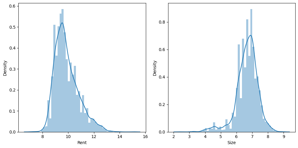
In order to lessen data skewness, this code applies a log transformation to the “Rent” and “Size” columns using np.log1p. The distribution of values in each column is then shown on distribution plots for the log-transformed numeric columns. For side-by-side visualization, the subplots are set up in a 1×2 grid, and ‘plt.tight_layout()’ makes sure there is enough space between each subplot. Lastly, the distribution plots’ subplots are displayed with ‘plt.show()’.

One-Hot Encoding Categorical Columns

Python3

cat_cols = ['Area Type', 'City', 'Furnishing Status',
            'Point of Contact', 'Tenant Preferred']

for col in cat_cols:
    temp = pd.get_dummies(df[col]).astype('int')
    df = pd.concat([df, temp], axis=1)

df.drop(cat_cols, axis=1, inplace=True)
print(df.head())

Output:

   BHK      Rent      Size  Bathroom  Built Area  Carpet Area  Super Area  \
0    2  9.210440  7.003974         2           0            0           1   
1    2  9.903538  6.685861         1           0            0           1   
2    2  9.741027  6.908755         1           0            0           1   
3    2  9.210440  6.685861         1           0            0           1   
4    2  8.922792  6.746412         1           0            1           0   
   Bangalore  Chennai  Delhi  ...  Mumbai  Furnished  Semi-Furnished  \
0          0        0      0  ...       0          0               0   
1          0        0      0  ...       0          0               1   
2          0        0      0  ...       0          0               1   
3          0        0      0  ...       0          0               0   
4          0        0      0  ...       0          0               0   
   Unfurnished  Contact Agent  Contact Builder  Contact Owner  Bachelors  \
0            1              0                0              1          0   
1            0              0                0              1          0   
2            0              0                0              1          0   
3            1              0                0              1          0   
4            1              0                0              1          1   
   Bachelors/Family  Family  
0                 1       0  
1                 1       0  
2                 1       0  
3                 1       0  
4                 0       0  
[5 rows x 22 columns]

One hot encoding is considered as the best practice to convert categorical columns into numerical ones as in this process none of the category is provided any preference that happens in the ordinal encoding method.

Splitting Data

Now we will split the whole data into training and validation part by using the 85:15 ratio.

Python3

# Splitting the Dataset
features = df.drop('Rent', axis=1)  # Features (independent variables)
target = df['Rent']  # Target variable (dependent variable)

# Splitting the data into training and validation sets
X_train, X_val, Y_train, Y_val = train_test_split(
    features, target, random_state=2023, test_size=0.15)

# Display the shapes of the training and validation sets
X_train.shape, X_val.shape

Output:

((4034, 21), (712, 21))

Model Development

Now as we are completely ready with the data part it’s preprocessing and splitting into training and the testing data. Now we will import catboostregressor from teh catboost module and train it on our dataset.

Python3

# CatBoost Regression Model
from catboost import CatBoostRegressor

# Initialize the CatBoostRegressor with RMSE as the loss function
model = CatBoostRegressor(loss_function='RMSE')

# Fit the model on the training data with verbose logging every 100 iterations
model.fit(X_train, Y_train, verbose=100)

Output:

Learning rate set to 0.051037
0:    learn: 0.8976462    total: 47.1ms    remaining: 47s
100:    learn: 0.3741647    total: 123ms    remaining: 1.09s
200:    learn: 0.3571139    total: 199ms    remaining: 792ms
300:    learn: 0.3455686    total: 275ms    remaining: 638ms
400:    learn: 0.3369937    total: 352ms    remaining: 526ms
500:    learn: 0.3305270    total: 430ms    remaining: 428ms
600:    learn: 0.3252100    total: 513ms    remaining: 340ms
700:    learn: 0.3200064    total: 623ms    remaining: 266ms
800:    learn: 0.3153692    total: 698ms    remaining: 173ms
900:    learn: 0.3116973    total: 773ms    remaining: 84.9ms
999:    learn: 0.3082544    total: 847ms    remaining: 0us
<catboost.core.CatBoostRegressor at 0x7fad65983730>

As we can see that the training has been done for around 1000 epochs and now we can use the training and validation data to analyze the performance of the model.

Let’s understand this code in detail:

‘CatBosstRegressor‘ is a python class provided by the catboost library for creating regression models. It is specifically designed for regression tasks, where the code is to predict a continuous numeric target variable on input features.

Here, in the code ‘CatBoostRegressor(loss function=’RMSE’) initializes catboost regression model with the Root Mean Squared Error(RMSE) as the loss function. The model aims to minimize the error during training.

‘Model.fit()’ method is used to train a model on the given dataset. In this model, it is applied to CatboostRegressor model. Here,

X_train: Feature matrix containing independent variables used for training.
Y_train: The target variable, which is the actual values the model aims to predict.
verbose=100: The verbose parameter controls the level of output displayed during training. In this code, ‘verbose=100’ specifies that the training process should provide verbose output, printing progress information every 100 iterations.

Together, these tools make it possible to build and train a CatBoost regression model with RMSE as the loss function. The model is trained using the supplied training data (X_train and Y_train), with verbose logging turned on to track the training status. The model can be used to make predictions on new data after training is finished.

Prediction

Python3

# Import the mean squared error (MSE) function from sklearn and alias it as 'mse'
from sklearn.metrics import mean_squared_error as mse

# Generate predictions on the training and validation sets using the trained 'model'
y_train = model.predict(X_train)
y_val = model.predict(X_val)

# Calculate and print the Root Mean Squared Error (RMSE) for training and validation sets
print("Training RMSE: ", np.sqrt(mse(Y_train, y_train)))
print("Validation RMSE: ", np.sqrt(mse(Y_val, y_val)))

Output:

Training RMSE:  0.308254377636178
Validation RMSE:  0.39986332453193907

Above we have seen that before passing the data to the model we have converted the categorical features to the numerical or one hot encoded one. But while we are using the catboost model we can choose not to perform this operation explicitly.

Conclusion

In this regression study employing CatBoost, we took advantage of the CatBoostRegressor’s capacity to forecast continuous numerical values from structured data. The preprocessing phase is made simpler by CatBoost’s skillful handling of categorical information. We set up the model hyperparameters carefully, made sure the training and validation procedures worked, and prepared the data methodically. We created a robust regression model by using feature engineering to assess the model’s performance using measures like RMSE. For precise regression predictions across a variety of structured datasets, CatBoost’s automatic category encoding, regularization techniques, and gradient boosting power make it an appealing option.