Google Sheets is a must for storing data in cells. These sheets are free online software. You can create and edit spreadsheets online and share them with many team members through the browser without using the MS Office suite. It is perfect for you to collaborate in real time.
Multiple team members can simultaneously work on the same sheet and save everything automatically. Working on the sheet will save a lot of your valuable time. Here are a few tips that you can follow to use the spreadsheet like a wizard.
Link: https://www.google.com/sheets/about/

Tips and Tricks to Use Google Sheets
Here are some tricks and tips that you can use on Google Sheets and make your work much easier:
1. Freeze Rows and Columns
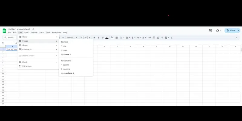
The most helpful trick and tip that you can use in Google Sheets is to freeze the columns and rows. When you are working on a massive volume of data, you want to see the column names, so you can freeze the top column to make it appear even when you scroll down.
The freeze function will pin the data in one place so you can always see it on the screen despite going up or down. The best thing is that you do not have to scroll up to read the column names.
You can freeze rows and columns following this procedure:
- Select the cell in the column or row you want to freeze.
- Go to the View menu, select Freeze, and select the appropriate option. If you have chosen to freeze a single row or column, you can notice the frozen row(s) or column(s).
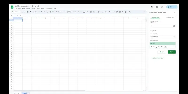
With conditional formatting, you can easily track the KPIs using colored cells. You can change the color of a row, column, or cell if the data meets some conditions, but only if the word or number in the cell contains the given word or number. It makes the spreadsheet dynamic and makes you read the content with ease.
For instance, you can format a spreadsheet so that it would be easy to highlight the poor performance of employees you have put in the sheet, low grades, or minus numbers obtained after doing the calculations.
You can do the conditional formatting by following these steps:
- You can open the spreadsheet using Google Sheets.
- Select the total number of cells you want to apply conditional formatting.
- Click Format→Conditional formatting.
- On the pop-up menu, add a rule:
- Single color – Under the format cells if you select the condition. Under formatting style, you can choose the color and style of the text or the cell.
- Color scale- Under preview, you can select the color scale. Set the color to minimum and maximum values.
- Click Done.
3. Use Alternate Colors
Another trick that you can save a lot of time when working on the spreadsheet is using alternate colors. You can add alternate colors to the rows instead of coloring manually, which can be done in two ways.
The first is to click the Format option from the menu on the top and then select alternating colors. Choose the default template or custom header colors and alternating colors in a row.
4. Make Use of Add-ons
Add-ons can be run inside Google Docs, Sheets, and Forms. These are tiny programs that developers use to do more on the spreadsheet. With this, you can easily add sidebars and quickly connect to many Google services.
You can navigate to Add-ons from the sheet and search for your desired add-on. You can find a lot of add-ons that you can easily connect to the spreadsheet. You can also import data to the data source and schedule emails.
5. Make use of a Template
Templates are an ideal way to save time when working alone or in a group with a G suite. It is not easy for you to recreate a report or newsletter; whenever you start creating a new report, it is not possible. Many time-saving templates offered by Google let you use the documents instead of struggling to put all of them together.
- Navigate to the home screen that is inside the Google Sheets.
- Pick the template of your choice.
- Click the Template gallery.
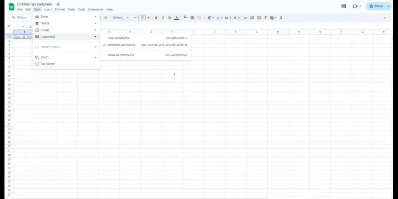
Google Sheets lets you leave a note or a comment in the cell. You can use the Note function to leave the note like you do with the comment function in Excel. With the help of notes, it becomes easy for you to add information about a cell.
Notes will help you add complexity to the spreadsheet. Many users ignore reading the notes as it leaves a small mark. However, you can use this for personal use.
You can use the comment function if multiple users work on the same sheet and in different locations. It allows you to make changes back and forth without changing the content. The comment function is suitable for editors. Using this, they can edit the content of their colleagues and improvise it.
7. Check Version History
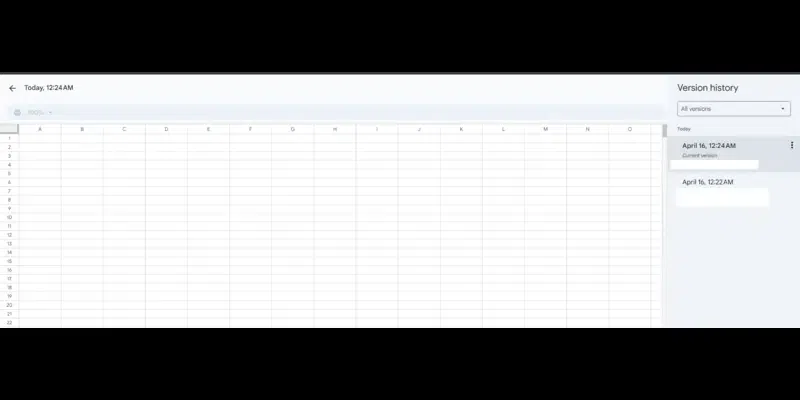
Users can edit the File and check the history to see the changes made. You can also check the changes made by other people using their names and the revision history. You can revert to the version you want and check the edits made by the person.
- Now open the Google Sheets.
- Go to the File and then select version history.
- Click on all changes saved in Drive in the menu bar.
- View the detailed revision in the revision history panel.
- Select the timestamp to check out the previous versions and see who has done the edits.
- Check the text highlighted in a different color and the deleted content that is struck off.
- Use the restore this version option to restore the File to the version you want.
- Click the back arrow to return to the current version.
Using the sum formula, you can easily add the values in the cells. You can select SUM from the drop-down list of Functions, or you can enter the formula by typing =SUM. You can hold the shift key to select the cells and add them together or add values between parentheses and press enter.
=SUM(B2:B6)
9. SUMIF
It is a must have in the Google Sheet formula list. The Sumif formula will let you sum the values in the cells only if certain conditions are met. It is easy to select Sumif from the math men you find in the formula drop-down list. You can also enter = Sumif in the empty cell and set the condition saying that if the value is less than or greater than this value, then add. Once the condition is set and the cells you want to add between parentheses, press enter.
Sumif (A:A, “text”, B:B)
10. Average
The average formula will let you get the average of the data in the selected cell range. It is easy to find the average of cells in one column or row (or).
You can also add random cells and put them together. In the empty cell, you can select AVERAGE from the function drop-down or enter =AVERAGE in the cell. You can select the cells whose average you want to take or manually enter the values to take the average.
Average (A: A)
11. Sort
The sort Google sheet advanced formula will be used to sort the cells with numerical data in ascending and descending order.
You can use the sort formula by typing =SORT in the empty cell, or you can click on the cell and then select SORT from the filter menu in the formula list. Select the range of cells you want to sort and press enter. It will reorder the data instantly.
12. TEXT
You can add this to the Google Sheets formula cheat sheet. The text formula will convert the cells that contain currency, decimals, and dates into the text format. You can use this formula by typing
=TEXT.
Otherwise, you can select the TEXT from the text menu in the formula list. You can enter the format in which you want to change the value between parentheses to text and press enter. If you are going to convert 20 USD to 20.00, you can use this formula – TEXT(A1,”0.00”)
Conclusion
You can make the most out of the Google Sheets by following the tips above. It is a combo of formulas and formatting options. Using these tips, you can customize the sheet briskly. The best thing is that you can create a template of the sheet you have formatted and can use this sheet for regular tasks you carry out on sheets.
FAQs – Google Sheets
Can I access Google Sheets offline?
Google Sheets will also work offline, which allows you to edit and view spreadsheets without connecting to the internet. You can enable offline access on Drive. Once you are offline, you can make changes; when you go offline, all the changes will be synced.
How can I protect the data on Google Sheets?
You can have two-factor authentication for the account for additional security. You can also set permissions for those who can view, edit, and comment on the sheet.
Can we automate some tasks on Google Sheets?
Yes, Google Sheets has automation capabilities. The best way to automate this is through macros. Using this, you can record the steps in the spreadsheet and use them to perform repetitive tasks.
How can Google sheet formulas be compared with Excel formulas?
The Google sheet formulas will be similar to the Excel functionality, such as SUM, VLOOKUP, and AVERAGE. Google Sheets offers cloud-based benefits like collaboration and integration with Google Workspace tools that are useful for the sales team.
Can Google Sheets be used for large datasets?
Yes, you can use Google Sheets for large datasets. However, it would help if you used formulas like ARRAY FORMULA to keep processing lag at bay. You can use IMPORT RANGE to consolidate the data and FILTER to segment the dataset to boost performance.
Share your thoughts in the comments
Please Login to comment...