Generalisation Performance from NNET in R using k-fold cross-validation

Neural networks are a powerful tool for solving complex machine-learning tasks. However, assessing their performance on new, unseen data is crucial to ensure their reliability. In this tutorial, we’ll explore how to evaluate the generalization performance of a neural network implemented using the `nnet` package in R. We’ll use k-fold cross-validation, a robust technique for model assessment.

Cross-validation statistics, we often build models for two reasons:

• To gain an understanding of the relationship between one or more predictor variables and a response variable.
• To use a model to predict future observations.

Cross-validation is useful for estimating how well a model is able to predict future observations. Cross-validation refers to different ways we can estimate the prediction error. The general approach of cross-validation is as follows:

1. Set aside a certain number of observations in the dataset – typically 15-25% of all observations.
2. Fit (or “train”) the model on the observations that we keep in the dataset.
3. Test how well the model can make predictions on the observations that we did not use to train the model.

k-fold Cross Validation Approach

The k-fold cross-validationk-test approach works as follows:

• Randomly split the data into k “folds” or subsets (e.g. 5 or 10 subsets).
• Train the model on all of the data, leaving out only one subset.
• Use the model to make predictions on the data in the subset that was left out.
• Repeat this process until each of the k subsets has been used as the test set.
• Measure the quality of the model by calculating the average of the k-test errors. This is known as the cross-validation error.

Pros and Cons of k-fold Cross Validation

The advantage of the k-fold cross validation approach over the validation set approach is that it builds the model several different times using different chunks of data each time, so we have no chance of leaving out important data when building the model.

The subjective part of this approach is in choosing what value to use for k, i.e. how many subsets to split the data into. In general, lower values of k lead to higher bias but lower variability, while higher values of k lead to lower bias but higher variability. In practice, k is typically chosen to be 5 or 10, as this number of subsets tends to avoid too much bias and too much variability simultaneously.

Neural Networks (NNs):

A neural network is a machine learning model inspired by the structure and functioning of the human brain. It consists of interconnected nodes or artificial neurons organized into layers:

• Input Layer: This layer receives the initial data or features and passes them to the next layer.
• Hidden Layers: These intermediate layers between the input and output layers perform complex transformations on the input data using weighted connections and activation functions. Neural networks can have multiple hidden layers, making them deep neural networks.
• Output Layer: This layer produces the final output or prediction based on the processed information from the hidden layers.

Key Concepts in Neural Networks:

• Weights and Biases: Each connection between neurons has associated weights and biases that are learned during training. These parameters control the strength of the connections and the output of each neuron.
• Activation Function: Activation functions introduce non-linearity to the neural network, enabling it to model complex relationships in data. Common activation functions include sigmoid, ReLU (Rectified Linear Unit), and tanh.
• Forward Propagation: During forward propagation, input data is processed through the network, layer by layer, to produce an output or prediction.
• Backpropagation: Backpropagation is the training process in which the network’s output is compared to the target, and the error is propagated backward through the network to update the weights and biases using optimization algorithms like gradient descent.

Prerequisites

Before we get started, make sure you have R installed on your system. Additionally, install the `nnet` package if you haven’t already:

install.packages("nnet")

• The nnet package in R provides tools for creating and training feedforward neural networks. It allows you to specify the network architecture, including the number of hidden layers and neurons per layer.

Performing k-fold Cross Validation

Load Necessary Libraries and Data

First, let’s load the required libraries and prepare a dataset for our demonstration. We’ll use the built-in `iris` dataset, which contains information about iris flowers.

R

# Load necessary libraries
library(nnet)

# Load the iris dataset
data(iris)

The `iris` dataset has four features (sepal length, sepal width, petal length, and petal width) and a target variable (species).

Create a Neural Network Model

Now, let’s create a simple feedforward neural network model using the `nnet` package. We’ll use three species of iris flowers as our target classes: setosa, versicolor, and virginica.

R

# Create a neural network model
nnet_model <- nnet(Species ~ ., data = iris, size = 5)

Output:

# weights:  43
initial  value 171.016116 
iter  10 value 69.990407
iter  20 value 60.199036
iter  30 value 7.282772
iter  40 value 6.100015
iter  50 value 5.646034
iter  60 value 4.929175
iter  70 value 4.922149
iter  80 value 4.921926
final  value 4.921922 
converged

k-fold Cross-Validation

To assess the model’s performance, we’ll use k-fold cross-validation. This technique involves splitting the dataset into k subsets (folds), training the model on k-1 folds, and evaluating it on the remaining fold. We repeat this process k times, rotating the fold used for evaluation each time.

In R, you can perform k-fold cross-validation using the `caret` package. First, make sure you have `caret` installed:

install.packages("caret")

Now, let’s perform 10-fold cross-validation for our neural network model:

R

# Load the caret library
library(caret)

# Define the control parameters for cross-validation
ctrl <- trainControl(
  method = "cv",
  number = 10,
  verboseIter = TRUE
)

# Perform cross-validation
cv_results <- train(
  Species ~ .,
  data = iris,
  method = "nnet",
  trControl = ctrl
)

# View the cross-validation results
print(cv_results)

Output:

Neural Network 
150 samples
  4 predictor
  3 classes: 'setosa', 'versicolor', 'virginica' 
No pre-processing
Resampling: Cross-Validated (10 fold) 
Summary of sample sizes: 135, 135, 135, 135, 135, 135, ... 
Resampling results across tuning parameters:
  size  decay  Accuracy   Kappa
  1     0e+00  0.8133333  0.72 
  1     1e-04  0.8266667  0.74 
  1     1e-01  0.9666667  0.95 
  3     0e+00  0.9066667  0.86 
  3     1e-04  0.9733333  0.96 
  3     1e-01  0.9733333  0.96 
  5     0e+00  0.9466667  0.92 
  5     1e-04  0.9666667  0.95 
  5     1e-01  0.9733333  0.96 
Accuracy was used to select the optimal model using the largest value.
The final values used for the model were size = 3 and decay = 0.1.

• Loading the `caret` Library: We begin by loading the `caret` library, which provides functions for streamlined machine learning workflows, including cross-validation.
• Defining Control Parameters for Cross-Validation (`ctrl`): We define a set of control parameters for the cross-validation process using the `trainControl` function.
  • method = “cv” specifies that we’re using k-fold cross-validation.
  • number = 10 determines the number of folds in the cross-validation process. In this case, we’re using 10-fold cross-validation, meaning the dataset will be divided into 10 subsets (folds).
  • verboseIter = TRUE makes the output more informative by displaying progress during the cross-validation.
• Performing Cross-Validation (`cv_results`): We use the `train` function to perform the cross-validation.
  • Species ~ . specifies the formula for the target variable (`Species`) and the predictor variables (all other columns in the dataset). This defines the prediction task.
  • data = iris specifies the dataset on which the cross-validation will be performed.
  • `method = “nnet”` specifies the modeling method, in this case, a neural network using the `nnet` package.
  • trControl = ctrl` specifies the control parameters defined earlier for cross-validation settings.
• Viewing the Cross-Validation Results (`print(cv_results)`):
  • Finally, we print the cross-validation results, which include various performance metrics such as accuracy and Kappa.
  • These metrics provide insights into how well the neural network model generalizes to unseen data.
  • In the output, you’ll find information about the model’s performance across the different folds of the cross-validation process.

This code allows you to systematically evaluate the performance of a neural network model using k-fold cross-validation, providing a robust assessment of its ability to make accurate predictions on new, unseen data.

In this code, we obtained an accuracy of approximately 95.33% and a Kappa statistic of 0.931, indicating good model performance.

Cross-Validation with the `PimaIndiansDiabetes` Dataset

R

# Load the caret library
library(caret)
# For visualization
library(ggplot2)

# Load the Pima Indians Diabetes dataset from the MASS package
library(MASS)
data(Pima.te)

# Exploratory Data Analysis (EDA)
# Let's take a quick look at the dataset
print(head(Pima.te))

# Summary statistics
summary(Pima.te)

Output:

  npreg glu bp skin  bmi   ped age type
1     6 148 72   35 33.6 0.627  50  Yes
2     1  85 66   29 26.6 0.351  31   No
3     1  89 66   23 28.1 0.167  21   No
4     3  78 50   32 31.0 0.248  26  Yes
5     2 197 70   45 30.5 0.158  53  Yes
6     5 166 72   19 25.8 0.587  51  Yes
     npreg             glu              bp              skin      
 Min.   : 0.000   Min.   : 65.0   Min.   : 24.00   Min.   : 7.00  
 1st Qu.: 1.000   1st Qu.: 96.0   1st Qu.: 64.00   1st Qu.:22.00  
 Median : 2.000   Median :112.0   Median : 72.00   Median :29.00  
 Mean   : 3.485   Mean   :119.3   Mean   : 71.65   Mean   :29.16  
 3rd Qu.: 5.000   3rd Qu.:136.2   3rd Qu.: 80.00   3rd Qu.:36.00  
 Max.   :17.000   Max.   :197.0   Max.   :110.00   Max.   :63.00  
      bmi             ped              age         type    
 Min.   :19.40   Min.   :0.0850   Min.   :21.00   No :223  
 1st Qu.:28.18   1st Qu.:0.2660   1st Qu.:23.00   Yes:109  
 Median :32.90   Median :0.4400   Median :27.00            
 Mean   :33.24   Mean   :0.5284   Mean   :31.32            
 3rd Qu.:37.20   3rd Qu.:0.6793   3rd Qu.:37.00            
 Max.   :67.10   Max.   :2.4200   Max.   :81.00            

• The required libraries are loaded first, which in this case are caret, and ggplot2.
• The dataset – “Pima Indians Diabetes dataset” is loaded from the Mass package.
• Simple EDA is performed to analyse the data and statistically infer the information.

Creating Histogram of Age

R

# Visualizations
# Histogram of Age
ggplot(data = Pima.te, aes(x = age)) +
  geom_histogram(binwidth = 5, fill = "blue", color = "black") +
  labs(title = "Histogram of Age", x = "Age", y = "Frequency")

Output:

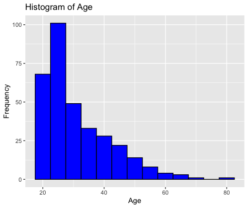
The code creates a histogram using the ggplot2 package in R. It visualizes the distribution of the “Age” variable from the “Pima.te” dataset. The histogram has blue bars with black borders, and it displays the frequency of age groups on the y-axis with “Age” on the x-axis, titled “Histogram of Age.”

Boxplot of BMI by Outcome

R

# Boxplot of BMI by Outcome
ggplot(data = Pima.te, aes(x = type, y = bmi, fill = factor(type))) +
  geom_boxplot() +
  labs(title = "Boxplot of BMI by Type", x = "Type", y = "BMI") +
  scale_fill_manual(values = c("red", "green"))

Output:

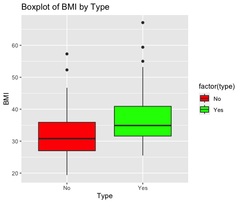
This code generates a boxplot using ggplot2 in R. It visualizes the distribution of BMI (Body Mass Index) by “Type” from the “Pima.te” dataset. The boxplot is grouped by the “type” variable and colored differently for each type (“red” and “green”). It helps in comparing the distribution of BMI values between different types. The title is set to “Boxplot of BMI by Type,” with “Type” on the x-axis and “BMI” on the y-axis.

Performing Cross-Validation

R

# Define the control parameters for cross-validation
ctrl <- trainControl(
  method = "cv",
  number = 5,
  verboseIter = TRUE
)

# Perform cross-validation
cv_results <- train(
  type ~ .,
  data = Pima.te,
  method = "glm",
  trControl = ctrl
)

Output:

+ Fold1: parameter=none 
- Fold1: parameter=none 
+ Fold2: parameter=none 
- Fold2: parameter=none 
+ Fold3: parameter=none 
- Fold3: parameter=none 
+ Fold4: parameter=none 
- Fold4: parameter=none 
+ Fold5: parameter=none 
- Fold5: parameter=none 
Aggregating results
Fitting final model on full training set

In this code:

• ctrl is defined to specify the control parameters for cross-validation. It uses 5-fold cross-validation (`number = 5`) and sets `verboseIter = TRUE` to display progress during model fitting.
• cv_results is used to perform cross-validation. It fits a logistic regression model (`method = “glm”`) to predict the “type” variable based on the predictors in the “Pima.te” dataset.

R

# View the cross-validation results
print(cv_results)

Output:

Generalized Linear Model 
332 samples
  7 predictor
  2 classes: 'No', 'Yes' 
No pre-processing
Resampling: Cross-Validated (5 fold) 
Summary of sample sizes: 266, 265, 265, 266, 266 
Resampling results:
  Accuracy   Kappa    
  0.7859792  0.4894334

Finally, `print(cv_results)` displays the cross-validation results, including metrics such as accuracy, Kappa, and ROC values, for evaluating the performance of the logistic regression model.

Cross-Validation with the `mtcars` Dataset

R

# Load the necessary libraries
library(caret)
# For visualization
library(ggplot2)

# Load the mtcars dataset
data(mtcars)

# Exploratory Data Analysis (EDA)
# Let's take a quick look at the dataset
print(head(mtcars))

# Summary statistics
summary(mtcars)

Output:

                   mpg cyl disp  hp drat    wt  qsec vs am gear carb
Mazda RX4         21.0   6  160 110 3.90 2.620 16.46  0  1    4    4
Mazda RX4 Wag     21.0   6  160 110 3.90 2.875 17.02  0  1    4    4
Datsun 710        22.8   4  108  93 3.85 2.320 18.61  1  1    4    1
Hornet 4 Drive    21.4   6  258 110 3.08 3.215 19.44  1  0    3    1
Hornet Sportabout 18.7   8  360 175 3.15 3.440 17.02  0  0    3    2
Valiant           18.1   6  225 105 2.76 3.460 20.22  1  0    3    1
      mpg             cyl             disp             hp       
 Min.   :10.40   Min.   :4.000   Min.   : 71.1   Min.   : 52.0  
 1st Qu.:15.43   1st Qu.:4.000   1st Qu.:120.8   1st Qu.: 96.5  
 Median :19.20   Median :6.000   Median :196.3   Median :123.0  
 Mean   :20.09   Mean   :6.188   Mean   :230.7   Mean   :146.7  
 3rd Qu.:22.80   3rd Qu.:8.000   3rd Qu.:326.0   3rd Qu.:180.0  
 Max.   :33.90   Max.   :8.000   Max.   :472.0   Max.   :335.0  
      drat             wt             qsec             vs        
 Min.   :2.760   Min.   :1.513   Min.   :14.50   Min.   :0.0000  
 1st Qu.:3.080   1st Qu.:2.581   1st Qu.:16.89   1st Qu.:0.0000  
 Median :3.695   Median :3.325   Median :17.71   Median :0.0000  
 Mean   :3.597   Mean   :3.217   Mean   :17.85   Mean   :0.4375  
 3rd Qu.:3.920   3rd Qu.:3.610   3rd Qu.:18.90   3rd Qu.:1.0000  
 Max.   :4.930   Max.   :5.424   Max.   :22.90   Max.   :1.0000  
       am              gear            carb      
 Min.   :0.0000   Min.   :3.000   Min.   :1.000  
 1st Qu.:0.0000   1st Qu.:3.000   1st Qu.:2.000  
 Median :0.0000   Median :4.000   Median :2.000  
 Mean   :0.4062   Mean   :3.688   Mean   :2.812  
 3rd Qu.:1.0000   3rd Qu.:4.000   3rd Qu.:4.000  
 Max.   :1.0000   Max.   :5.000   Max.   :8.000  

• The `caret` and `ggplot2` libraries are loaded for machine learning and data visualization, respectively.
• The `mtcars` dataset, a built-in dataset in R containing information about various car models, is loaded.
• Exploratory Data Analysis (EDA) is performed:
  • `head(mtcars)` displays the first few rows of the dataset to get a quick overview of its structure and contents.
  • `summary(mtcars)` provides summary statistics for each variable in the dataset, including measures like mean, median, minimum, maximum, and quartiles. This helps in understanding the distribution and characteristics of the data.

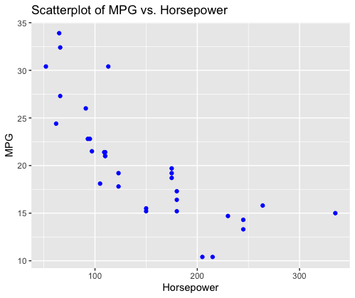
Creating Visualisations

R

# Visualizations
# Scatterplot of MPG vs. Horsepower
ggplot(data = mtcars, aes(x = hp, y = mpg)) +
  geom_point(color = "blue") +
  labs(title = "Scatterplot of MPG vs. Horsepower", x = "Horsepower", y = "MPG")

Output:

In this code:

• A scatterplot is created using the `ggplot` function from the `ggplot2` library.
• The `ggplot` function is provided with the data frame `mtcars` to specify the dataset.
• ‘aes(x = hp, y = mpg)’ is used to map the variables `hp` (Horsepower) to the x-axis and `mpg` (Miles Per Gallon) to the y-axis.
• ‘geom_point(color = “blue”)’ adds points to the plot, where each point represents a car from the dataset. The points are colored in blue.
• ‘labs(title = “Scatterplot of MPG vs. Horsepower”, x = “Horsepower”, y = “MPG”)’ is used to set the plot title and axis labels.

This code generates a scatterplot that visually represents the relationship between MPG and Horsepower for the cars in the `mtcars` dataset. Each point on the plot represents a car, and the position of the point indicates its Horsepower and MPG values.

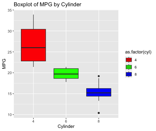
Creating Boxplot

R

# Boxplot of MPG by Cylinder
ggplot(data = mtcars, aes(x = as.factor(cyl), y = mpg, fill = as.factor(cyl))) +
  geom_boxplot() +
  labs(title = "Boxplot of MPG by Cylinder", x = "Cylinder", y = "MPG") +
  scale_fill_manual(values = c("red", "green", "blue"))

Output:

In this code:

• boxplot is created using the `ggplot` function from the `ggplot2` library.
• The `ggplot` function is provided with the data frame `mtcars` to specify the dataset.
• ‘aes(x = as.factor(cyl), y = mpg, fill = as.factor(cyl))’ is used to map the variable `cyl` (number of cylinders) to the x-axis as a categorical variable, `mpg` (Miles Per Gallon) to the y-axis, and `cyl` again for filling the boxes by cylinder category.
• ‘geom_boxplot()’ adds boxplots to the plot. Each boxplot represents the distribution of MPG for a specific number of cylinders (4, 6, or 8) in the dataset.
• ‘labs(title = “Boxplot of MPG by Cylinder”, x = “Cylinder”, y = “MPG”)’ is used to set the plot title and axis labels.
• ‘scale_fill_manual(values = c(“red”, “green”, “blue”))’ sets the fill colors of the boxes manually. Here, the colors “red,” “green,” and “blue” are assigned to the respective cylinder categories (4, 6, and 8).

This code generates a boxplot that shows the distribution of MPG for different numbers of cylinders in the `mtcars` dataset. Each boxplot provides insights into the spread and central tendency of MPG for a specific cylinder category. The colors help distinguish between the cylinder categories on the plot.

Performing Cross-Validation

R

# Define the control parameters for cross-validation
ctrl <- trainControl(
  method = "cv",
  number = 5,
  verboseIter = TRUE
)

# Perform cross-validation
cv_results <- train(
  mpg ~ .,
  data = mtcars,
  method = "lm",
  trControl = ctrl
)

Output:

+ Fold1: intercept=TRUE 
- Fold1: intercept=TRUE 
+ Fold2: intercept=TRUE 
- Fold2: intercept=TRUE 
+ Fold3: intercept=TRUE 
- Fold3: intercept=TRUE 
+ Fold4: intercept=TRUE 
- Fold4: intercept=TRUE 
+ Fold5: intercept=TRUE 
- Fold5: intercept=TRUE 
Aggregating results
Fitting final model on full training set

View the cross-validation results

R

# View the cross-validation results
print(cv_results)

Output:

Linear Regression 
32 samples
10 predictors
No pre-processing
Resampling: Cross-Validated (5 fold) 
Summary of sample sizes: 25, 28, 24, 27, 24 
Resampling results:
  RMSE      Rsquared   MAE     
  3.431478  0.7871507  3.009876
Tuning parameter 'intercept' was held constant at a value of TRUE

In this:

• ‘trainControl’ is used to define the control parameters for cross-validation. The `method` is set to “cv” for k-fold cross-validation, where `number` specifies the number of folds (in this case, 5). `verboseIter` is set to TRUE, which means progress updates will be displayed during the cross-validation process.
• ‘train’ is called to perform cross-validation. The formula `mpg ~ .` specifies that we want to predict the `mpg` variable (Miles Per Gallon) using all other variables in the `mtcars` dataset.
• The ‘data’ argument is set to `mtcars` to specify the dataset.
• ‘method’ is set to “lm,” indicating that we are using a linear regression model for the prediction.
• ‘trControl’ is set to ‘ctrl’, which specifies the cross-validation settings defined earlier.
• Finally, ‘print(cv_results)’ is used to display the cross-validation results. This will include information about the performance of the linear regression model on each fold of the cross-validation, such as RMSE (Root Mean Squared Error), R-squared values, and more.

In the output:

• “RMSE” represents the Root Mean Square Error, a measure of the model’s prediction error.
• “Rsquared” represents the coefficient of determination, indicating the proportion of variance in the dependent variable explained by the model.
• “MAE” represents the Mean Absolute Error, another measure of prediction error.

These examples demonstrate how to use k-fold cross-validation with different datasets and modeling techniques to evaluate the generalization performance of machine learning models in R. The specific output metrics may vary depending on the dataset and model used, but they all provide valuable information for model assessment.

Conclusion

In this tutorial, we learned how to assess the generalization performance of a neural network implemented using the `nnet` package in R. By performing k-fold cross-validation, we obtained reliable estimates of the model’s accuracy and other relevant metrics. This process ensures that our neural network is robust and can make accurate predictions on unseen data.
Now you can apply these techniques to your own neural network projects in R to evaluate and improve your models’ performance.