Adjusted Coefficient of Determination in R Programming

Prerequisite: Multiple Linear Regression using R

A well-fitting regression model produces predicted values close to the observed data values. The mean model, which uses the mean for every predicted value, commonly would be used if there were no informative predictor variables. The fit of a proposed regression model should therefore be better than the fit of the mean model. The three most common statistical measures used to evaluate regression model fit are:

1. Coefficient of determination (R²), Adjusted R² 
2. Root Mean Squared Error (RMSE)
3. Overall F-test

So in this article let’s discuss the adjusted coefficient of determination or adjusted R² in R programming. Much like the coefficient of the determination itself, R²_adj  describes the variance of the response variable y, which may be predicted on the basis of the independent feature variables, x. However, two important distinctions:

1. R²_adj takes into account the number of variables in the data set. It penalizes for data points that do not fit the regression model developed.
2. An implication of the above statement would be that R²_adj, unlike R² does not increase continually with an increase in feature variables (due to change in its mathematical calculation) and, does not take into consideration independent variables that don’t affect the feature variable. This protects the model against overfitting.

This measure is therefore more suited for multiple regression models than R², which works only for the simple linear regression model.

Mathematical Formula

where,

n: number of data points

k: number of variables excluding the outcome

R²: coefficient of determination

Example

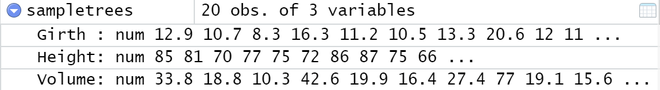
Input: A data set of 20 records of trees with labels height,girth and volume. Structure of the data set is given below.

Model 1: This model considers height and volume to predict girth

Model 2: This model considers only volume to predict girth

Output:

Model 1: R-squared:  0.9518,    Adjusted R-squared:  0.9461 
Model 2: R-squared:  0.9494,    Adjusted R-squared:  0.9466 

Explanation of results: Model 1 considers the label height as a variable that determines girth, which is not at all always true and hence, considers an irrelevant label in the model. The results of R-squared suggest Model 1 has a better fit, which is evidently not true. The metric adjusted R-squared, which is greater for Model 2 mitigates this anomaly.

Implementation in R

It is very easy to find out the Adjusted Coefficient of Determination in the R language. The steps to follow are:

• Make a data frame in R.
• Calculate the multiple linear regression model and save it in a new variable.
• The so calculated new variable’s summary has an adjusted coefficient of determination or adjusted R-squared parameter that needs to be extracted.

Example:

R

# R program to illustrate
# Adj Coefficient of determination

# Creating a dataframe
sample_data <- data.frame(col1 = c(10, 20, 30, 40, 50),
                          col2 = c(1, 2, 3, 2, 2),
                          col3 = c(10, 20, 30, 20, 25))

# multiple regression model
# where col1, col2 are features
sample_model <- lm(col3~col1 + col2,
                   data = sample_data)

# Extracting Adj R-squared parameter
# from summary
summary(sample_model)$adj.r.squared

Output:

[1] 0.9318182