Convolutional Neural Network (CNN) in Tensorflow
Last Updated :
02 Mar, 2022
It is assumed that the reader knows the concepts of Neural Networks and Convolutional Neural Networks. If you are sure about the topics please refer to Neural Networks and Convolutional Neural Networks.
Building Blocks of CNN:
Convolutional Neural Networks are mainly made up of three types of layers:
- Convolutional Layer: It is the main building block of a CNN. It inputs a feature map or input image consisting of a certain height, width, and channels and transforms it into a new feature map by applying a convolution operation. The transformed feature map consists of different height, width, and channels based on the filter_size, padding, and stride.
Python3
import tensorflow as tf
conv_layer = tf.keras.layers.Conv2D(
filters, kernel_size, strides=(1, 1), padding='valid',
data_format=None, dilation_rate=(1, 1), groups=1, activation=None,
use_bias=True, kernel_initializer='glorot_uniform',
bias_initializer='zeros', kernel_regularizer=None,
bias_regularizer=None, activity_regularizer=None, kernel_constraint=None,
bias_constraint=None, **kwargs
)
|
- Pooling Layer: Pooling layers do the operation of downsampling, where it reduces the size of the input feature map. Two main types of pooling are Max Pooling and Average Pooling.
Python3
import tensorflow as tf
max_pooling_layer = tf.keras.layers.MaxPool2D(
pool_size=(2, 2), strides=None, padding='valid', data_format=None,
**kwargs
)
avg_pooling_layer = tf.keras.layers.AveragePooling2D(
pool_size=(2, 2), strides=None, padding='valid', data_format=None,
**kwargs
)
|
Note: This article is mainly focused on image data. The suffix 2D at each layer name corresponds to two-dimensional data (images). If working on different dimensional data please refer to TensorFlow API.
- Fully-Connected Layer: Each node in the output layer connects directly to a node in the previous layer.
Python3
import tensorflow as tf
fully_connected_layer = tf.keras.layers.Dense(
units, activation=None, use_bias=True,
kernel_initializer='glorot_uniform',
bias_initializer='zeros', kernel_regularizer=None,
bias_regularizer=None, activity_regularizer=None, kernel_constraint=None,
bias_constraint=None, **kwargs
)
|
Here we have seen the basic building blocks of CNN, so now let’s see the implementation of a CNN model in TensorFlow.
Implementation of LeNet – 5:
LeNet – 5 is a basic convolutional neural network created for the task of handwritten digit recognition for postal codes.
- Loading MNIST Dataset: MNIST Dataset consists of 60,000 train images and 10,000 test images of shape 28 * 28.
Python3
from tensorflow.keras.datasets import mnist
(X_train, y_train), (X_test, y_test) = mnist.load_data()
print(f'X_train shape: {X_train.shape}, X_test shape: {X_test.shape}')
|
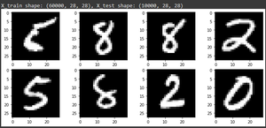
Plot Random Images
- Preprocessing Data: It includes normalizing the pixel values from 0 to 255 to 0 to 1. The labels for the images are 0 – 9. It is converted into a one-hot vector.
Python3
from tensorflow.keras.utils import to_categorical
X_train = X_train.astype('float32')
X_test = X_test.astype('float32')
X_train = X_train/255.0
X_test = X_test/255.0
X_train = X_train.reshape(X_train.shape[0], X_train.shape[1], X_train.shape[2], 1)
X_test = X_test.reshape(X_test.shape[0], X_test.shape[1], X_test.shape[2], 1)
y_train = to_categorical(y_train)
y_test = to_categorical(y_test)
|
Python3
from tensorflow.keras.models import Sequential
from tensorflow.keras.layers import Conv2D, MaxPooling2D, Dense, Flatten
model = Sequential()
model.add(Conv2D(filters=6, kernel_size=(5, 5), strides=1, activation = 'relu', input_shape = (32,32,1)))
model.add(MaxPooling2D(pool_size=(2, 2), strides = 2))
model.add(Conv2D(filters=16, kernel_size=(5, 5), strides=1, activation='relu'))
model.add(MaxPooling2D(pool_size = 2, strides = 2))
model.add(Flatten())
model.add(Dense(units=120, activation='relu'))
model.add(Dense(units=84, activation='relu'))
model.add(Dense(units=10, activation='softmax'))
model.compile(optimizer='adam', loss='categorical_crossentropy', metrics=['accuracy'])
|
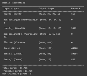
Model Summary
Python3
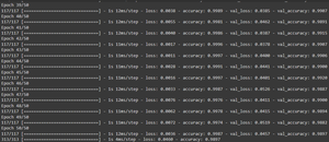
epochs = 50
batch_size = 512
history = model.fit(X_train, y_train, epochs=epochs, batch_size=batch_size,
steps_per_epoch=X_train.shape[0]//batch_size,
validation_data=(X_test, y_test),
validation_steps=X_test.shape[0]//batch_size, verbose = 1)
_, acc = model.evaluate(X_test, y_test, verbose = 1)
print('%.3f' % (acc * 100.0))
plt.figure(figsize=(10,6))
plt.plot(history.history['accuracy'], color = 'blue', label = 'train')
plt.plot(history.history['val_accuracy'], color = 'red', label = 'val')
plt.legend()
plt.title('Accuracy')
plt.show()
|
Training History
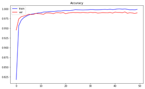
Epochs vs Accuracy
Results: LeNet-5 model has given the performance of 98.97% on the MNIST dataset.
The above task was image classification, but using Tensorflow we can perform tasks such as Object Detection, Image Localization, Landmark Detection, Style Transfer.
Share your thoughts in the comments
Please Login to comment...