Compute Empirical Cumulative Distribution Function in R

The empirical cumulative distribution function (ECDF) is a non-parametric way to estimate the cumulative distribution function (CDF) of a random variable. It is a step function that jumps up by 1/N at each observed data point, where N is the total number of data points. The ECDF is a useful tool for visualizing the distribution of a dataset and can provide insights into the underlying distribution that would be difficult to obtain through traditional summary statistics.

Related Concepts

Before diving into the details of the ECDF, let’s first define some related concepts:

The probability density function (PDF) is used to describe the probability distribution of a continuous random variable. The PDF is defined as the derivative of the cumulative distribution function:

where F(x) is the cumulative distribution function.

The probability mass function (PMF) is used to describe the probability distribution of a discrete random variable. The PMF gives the probability that a discrete random variable takes a certain value:

where X is the random variable and k is a particular value.

The cumulative distribution function is used to describe the probability that a random variable takes a value less than or equal to a certain value. The CDF is defined as:

Mathematical Concept of ECDF

The ECDF is defined as follows:

Let    be a random sample of size n from a distribution with CDF  . The ECDF is given by:

where  is the indicator function if   then, equal to 1 else 0 otherwise. In other words, the ECDF is the proportion of observations that are less than or equal to x.

The ECDF is a step function that jumps up by 1/n at each observed data point and is constant between data points. It starts at 0 and ends at 1, making it a useful tool for visualizing the distribution of a dataset.

Mean, Variance, Quantiles, and Confidence Intervals

The ECDF can be used to estimate the mean, variance, and quantiles of a distribution. The mean of the distribution can be estimated as the area under the curve of the ECDF:

The variance of the distribution can be estimated as:

The ECDF can also be used to estimate confidence intervals for the CDF, which can be useful for hypothesis testing and parameter estimation.

Properties of ECDF

The ECDF has several useful properties:

• It is a non-parametric estimate of the CDF, meaning it can be applied to a wide variety of distributions without making assumptions about their shape or parameters.
• It is consistent, meaning that as the sample size increases, the ECDF converges to the true CDF.
• It is unbiased, meaning that on average, the ECDF estimates the true CDF.
• It is a step function, which makes it useful for visualizing the distribution of a dataset.

Now, let’s move on to some examples of how to compute and plot the ECDF. Before starting this tutorial, you need to have a basic understanding of R language and its data structures. You should also have the latest version of R installed on your computer.

Steps

Step 1: Load the Data

The first step is to load the data into R. You can either import the data from an external file or create a sample data set in R. For the purpose of this tutorial, let’s create a sample data set in R.

R

data <- rnorm(1000, mean=50, sd=10)

Step 2: Compute the ECDF

The ECDF can be computed using the ecdf function from the stats library in R. The function takes the data set as an argument and returns the ECDF function.

R

library(stats)
ecdf_func <- ecdf(data)

Step 3: Plot the ECDF

The ECDF can be plotted using the plot function in R. The ECDF function returned by the ecdf function can be plotted by passing it as the first argument to the plot function.

You can customize the plot by adding labels, and titles, and changing the appearance of the plot.

R

plot(ecdf_func, xlab="Data", ylab="Cumulative Probability",
     main="Empirical Cumulative Distribution Function")

Output:

Empirical Cumulative Distribution Function Plot

Illustrations

Example 1: Computing and Plotting the ECDF for a Simple Dataset

Suppose we have a set of 10 data points: 1, 2, 3, 4, 4, 5, 6, 7, 8, and 9. We want to compute the ECDF of this data set.

Manually, we would first sort the data in ascending order: 1, 2, 3, 4, 4, 5, 6, 7, 8, 9. Then, for each value of x, we would count the number of observations that are less than or equal to x, and divide by the total number of observations.

For example, to compute the ECDF at x=5, we would count the number of observations that are less than or equal to 5, which is 6. Dividing by the total number of observations, we get . We would repeat this process for all values of x.
here’s the R implementation:

Step 1: Sort the data

The first step is to sort the data in ascending order and calculate the number of data points:

R

data <- c(1, 2, 5, 4, 4, 3, 6, 7, 8, 9)
sorted <- sort(data, decreasing = FALSE)
n = length(sorted)
paste('Length :', n)
print(sorted)

Output:

'Length : 10'
 [1] 1 2 3 4 4 5 6 7 8 9

Step 2: Compute the ECDF

To compute the ECDF, we need to loop over each data point in the sorted dataset, and calculate the proportion of data points that are less than or equal to that point:

R

# Define a function to compute the ECDF
ecdf_func <- function(data) {
    Length <- length(data)
    sorted <- sort(data)

    ecdf <- rep(0, Length)
    for (i in 1:n) {
        ecdf[i] <- sum(sorted <= data[i]) / Length
    }
    return(ecdf)
}

ecdf <- ecdf_func(data)
print(ecdf)

Output:

[1] 0.1 0.2 0.6 0.5 0.5 0.3 0.7 0.8 0.9 1.0

Step 3: Compute ECDF using ecdf() function

In R, we can compute the ECDF using the built-in ecdf() function:

R

ecdf_fun <- ecdf(data)
ecdf_ <- ecdf_fun(data)
print(ecdf_)

The output will be:

 [1] 0.1 0.2 0.6 0.5 0.5 0.3 0.7 0.8 0.9 1.0

Step 4:  Check whether both ecdf values are identical or not

R

# Check if the ECDF functions are identical
identical(ecdf, ecdf_)

Output:

TRUE

The two methods produce the same result, as can be seen by comparing the outputs of ecdf and ecdf_. The empirical cumulative distribution function assigns a probability of 0.1 to the smallest value in the data, a probability of 0.2 to the second smallest value, and so on. The largest value in the data has a probability of 1.0.

Step 6: Plot the ECDF

We can also plot the ECDF using the plot() function:

R

plot(data, ecdf_func(data), main="Custom Empirical Cumulative Distribution Plot", xlab="Data Points", ylab="ECDF Value")

Output

Custom Empirical Cumulative Distribution Function Plot

Example 2: ECDF of Normally distributed data

Suppose we have a dataset of 1000 observations that follows a normal distribution with a mean 0 and a standard deviation of 1. We want to compute the ECDF of this dataset and plot it.

Step 1: Generate the data

We generate a dataset of 100 observations that follows a normal distribution with mean 0 and standard deviation 1. In R, we can use the rnorm() function to generate random normal data:

R

set.seed(123)
data <- rnorm(100, mean = 0, sd = 1)

Here, we set the random seed to ensure reproducibility, and generate 1000 random numbers from a normal distribution with a mean of 0 and a standard deviation of 1. The resulting data object is a vector of length 100.

Step 2: Compute the ECDF values

For each value of x, we want to compute the estimated probability that a data point in the dataset is less than or equal to x. This can be done using the ECDF formula, which is denoted as \hat{F}(x) and defined as:  where n is the sample size,   are the observed data points, and   is the indicator function that is 1 if  is less than or equal to x, and 0 otherwise.

In R, we can compute the ECDF values manually using a for loop:

R

# Define a function to compute the ECDF
ecdf_func <- function(data) {
    Length <- length(data)
    sorted <- sort(data)

    ECDF <- rep(0, Length)
    for (i in 1:Length) {
        ECDF[i] <- sum(sorted <= data[i]) / Length
    }
    return(ECDF)
}

ecdf1 <- ecdf_func(data)
plot(data, ecdf1, xlab="Data", ylab="Cumulative Probability",
     main="Empirical Cumulative Distribution Function")

Output:

Empirical Cumulative Distribution Function

Step 3: Check with ecdf() function identical or not

R

ecdf_fun <- ecdf(data)
ecdf <- ecdf_fun(data)
# Check with ecdf() function identical or not
identical(ecdf1, ecdf)

Output:

TRUE

Step 4: Compute the cumulative normal distribution with new data

 First, we define a sequence of values for x. For each value of x, we want to compute the true probability that a standard normal random variable is less than or equal to x. This can be done using the standard normal CDF, and use the pnorm() function to compute the true CDF values for each value of x.  we use the same sample mean and standard deviation here also.

R

# Create a sequence dataset of 100 values
x <- seq(-4, 4, length.out = 100)
# Cumulative Normal distribution
prob <- pnorm(x, mean = 0, sd = 1)
plot(prob,  xlab="Data", ylab="Probability",
     main="Cumulative Normal Distribution")

Output:

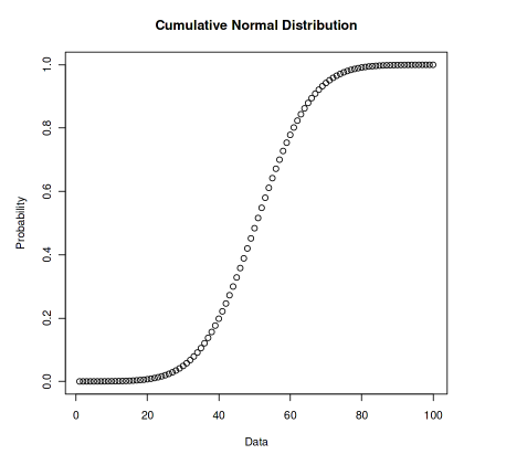
Cumulative Normal Distribution

Step 5: Compute ecdf for x using the function ecdf_fun() and Plot both cdf and ecdf on same plot

We can plot the true CDF values and ECDF values on the same plot to visualize how closely they match. Here, we use the plot() function to create a line plot with x-values from -4 to 4, and y-values corresponding to the true CDF values in blue and the ECDF values in red. We also add a legend to the plot to distinguish between the two lines.

R

ecdf = ecdf_fun(x)
plot(x, prob, type = "l", col = "blue", lwd = 2,
     xlab = "x", ylab = "Cumulative probability",
     main = "True CDF vs ECDF")
lines(x, ecdf, type = "l", col = "red", lwd = 2)
legend("bottomright", legend = c("True CDF", "ECDF"),
       col = c("blue", "red"), lwd = 2)

Output:

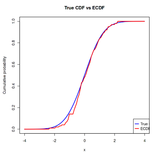
True CDF vs ECDF

We first generate the normal data using the rnorm() function. Then, we compute the sample mean and standard deviation using the mean() and sd() functions. We then define a sequence of values for x and use the pnorm() function to compute the true CDF values for each value of x. We also compute the ECDF manually using a for loop and the sum() function. Finally, we plot both the true CDF

Conclusion

Empirical Cumulative Distribution Function (ECDF) is a powerful statistical tool that allows us to visualize and analyze data by estimating the cumulative distribution function of a population. It is defined as the proportion of observations that are less than or equal to each value of x, and it can be computed manually or using code in R. The ECDF is a step function that interpolates linearly between data points, and it has several properties such as mean, variance, quantiles, and confidence intervals. By using the ECDF, we can gain insights into the distribution of data and make informed decisions based on the available data.