In this article, we will discuss how we perform Algebraic Operations on a Matrix in R Programming Language. so we will start with the matrix.
What is Matrix?
A Matrix is a rectangular arrangement of numbers in rows and columns. In a matrix, as we know rows are the ones that run horizontally and columns are the ones that run vertically. In R Programming Language matrices are two-dimensional, homogeneous data structures. These are some examples of matrices. 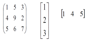
What are the Algebraic Operations?
Basic algebraic operations are any one of the traditional operations of arithmetic, which are addition, subtraction, multiplication, division, raising to an integer power, and taking roots. These operations may be performed on numbers, in which case they are often called arithmetic operations. We can perform many more algebraic operations on a matrix in R. Algebraic operations that can be performed on a matrix in R:
- Operations on a single matrix
- Unary operations
- Binary operations
- Linear algebraic operations
- Rank, determinant, transpose, inverse, trace of a matrix
- Nullity of a matrix
- Eigenvalues and eigenvectors of matrices
- Solve a linear matrix equation
Operations on a single matrix
We can use overloaded arithmetic operators to do element-wise operation on a matrix to create a new matrix. In case of +=, -=, *= operators, the existing matrix is modified.
R
a = matrix(
c(1, 2, 3, 4, 5, 6, 7, 8, 9),
nrow = 3,
ncol = 3,
byrow = TRUE
)
cat("The 3x3 matrix:\n")
print(a)
cat("Adding 1 to every element:\n")
print(a + 1)
cat("Subtracting 3 from each element:\n")
print(a-3)
cat("Multiplying each element by 10:\n")
print(a * 10)
cat("Squaring each element:\n")
print(a ^ 2)
cat("Doubled each element of original matrix:\n")
print(a * 2)
|
Output:
The 3x3 matrix:
     [, 1] [, 2] [, 3]
[1, ]    1    2    3
[2, ]    4    5    6
[3, ]    7    8    9
Adding 1 to every element:
     [, 1] [, 2] [, 3]
[1, ]    2    3    4
[2, ]    5    6    7
[3, ]    8    9   10
Subtracting 3 from each element:
     [, 1] [, 2] [, 3]
[1, ]   -2   -1    0
[2, ]    1    2    3
[3, ]    4    5    6
Multiplying each element by 10:
     [, 1] [, 2] [, 3]
[1, ]   10   20   30
[2, ]   40   50   60
[3, ]   70   80   90
Squaring each element:
     [, 1] [, 2] [, 3]
[1, ]    1    4    9
[2, ]   16   25   36
[3, ]   49   64   81
Doubled each element of original matrix:
     [, 1] [, 2] [, 3]
[1, ]    2    4    6
[2, ]    8   10   12
[3, ]   14   16   18
Unary operations
Many unary operations can be performed on a matrix in R. This includes sum, min, max, etc.
R
a = matrix(
c(1, 2, 3, 4, 5, 6, 7, 8, 9),
nrow = 3,
ncol = 3,
byrow = TRUE
)
cat("The 3x3 matrix:\n")
print(a)
cat("Largest element is:\n")
print(max(a))
cat("Smallest element is:\n")
print(min(a))
cat("Sum of elements is:\n")
print(sum(a))
|
Output:
The 3x3 matrix:
     [, 1] [, 2] [, 3]
[1, ]    1    2    3
[2, ]    4    5    6
[3, ]    7    8    9
Largest element is:
[1] 9
Smallest element is:
[1] 1
Sum of elements is:
[1] 45
Binary operations
These operations apply on a matrix elementwise and a new matrix is created. You can use all basic arithmetic operators like +, -, *, /, etc. In case of +=, -=, = operators, the existing matrix is modified.
R
a = matrix(
c(1, 2, 3, 4, 5, 6, 7, 8, 9),
nrow = 3,
ncol = 3,
byrow = TRUE
)
cat("The 3x3 matrix:\n")
print(a)
b = matrix(
c(1, 2, 5, 4, 6, 2, 9, 4, 3),
nrow = 3,
ncol = 3,
byrow = TRUE
)
cat("The another 3x3 matrix:\n")
print(b)
cat("Matrix addition:\n")
print(a + b)
cat("Matrix subtraction:\n")
print(a-b)
cat("Matrix element wise multiplication:\n")
print(a * b)
cat("Regular Matrix multiplication:\n")
print(a %*% b)
cat("Matrix elementwise division:\n")
print(a / b)
|
Output:
The 3x3 matrix:
     [, 1] [, 2] [, 3]
[1, ]    1    2    3
[2, ]    4    5    6
[3, ]    7    8    9
The another 3x3 matrix:
     [, 1] [, 2] [, 3]
[1, ]    1    2    5
[2, ]    4    6    2
[3, ]    9    4    3
Matrix addition:
     [, 1] [, 2] [, 3]
[1, ]    2    4    8
[2, ]    8   11    8
[3, ]   16   12   12
Matrix subtraction:
     [, 1] [, 2] [, 3]
[1, ]    0    0   -2
[2, ]    0   -1    4
[3, ]   -2    4    6
Matrix element wise multiplication:
     [, 1] [, 2] [, 3]
[1, ]    1    4   15
[2, ]   16   30   12
[3, ]   63   32   27
Regular Matrix multiplication:
     [, 1] [, 2] [, 3]
[1, ]   36   26   18
[2, ]   78   62   48
[3, ]  120   98   78
Matrix elementwise division:
          [, 1]      [, 2] [, 3]
[1, ] 1.0000000 1.0000000  0.6
[2, ] 1.0000000 0.8333333  3.0
[3, ] 0.7777778 2.0000000  3.0
Linear algebraic operations
One can perform many linear algebraic operations on a given matrix In R. Some of them are as follows:
Rank, determinant, transpose, inverse, trace of a matrix
- Rank: The rank of a matrix is the maximum number of linearly independent rows or columns in the matrix. In other words, it is the dimension of the column space (or equivalently, the row space) of the matrix.
- Determinant: The determinant has various geometric interpretations, such as measuring the volume scaling factor of a linear transformation represented by the matrix.
- Transpose: The transpose of a matrix is obtained by swapping its rows and columns.
- Inverse: The inverse of a square matrix is a matrix that, when multiplied with the original matrix, results in the identity matrix.
- Trace: The trace of a square matrix is the sum of its diagonal elements.
R
library(pracma)
library(psych)
A = matrix(
c(6, 1, 1, 4, -2, 5, 2, 8, 7),
nrow = 3,
ncol = 3,
byrow = TRUE
)
cat("The 3x3 matrix:\n")
print(A)
cat("Rank of A:\n")
print(Rank(A))
cat("Trace of A:\n")
print(tr(A))
cat("Determinant of A:\n")
print(det(A))
cat("Transpose of A:\n")
print(t(A))
cat("Inverse of A:\n")
print(inv(A))
|
Output:
The 3x3 matrix:
     [, 1] [, 2] [, 3]
[1, ]    6    1    1
[2, ]    4   -2    5
[3, ]    2    8    7
Rank of A:
[1] 3
Trace of A:
[1] 11
Determinant of A:
[1] -306
Transpose of A:
     [, 1] [, 2] [, 3]
[1, ]    6    4    2
[2, ]    1   -2    8
[3, ]    1    5    7
Inverse of A:
            [, 1]         [, 2]        [, 3]
[1, ]  0.17647059 -0.003267974 -0.02287582
[2, ]  0.05882353 -0.130718954  0.08496732
[3, ] -0.11764706  0.150326797  0.05228758
Nullity of a matrix
The nullity of a matrix is the dimension of the null space, also known as the kernel, of the matrix. The null space of a matrix.
R
library(pracma)
a = matrix(
c(1, 2, 3, 4, 5, 6, 7, 8, 9),
nrow = 3,
ncol = 3,
byrow = TRUE
)
cat("The 3x3 matrix:\n")
print(a)
col = ncol(a)
rank = Rank(a)
nullity = col - rank
cat("Nullity of matrix is:\n")
print(nullity)
|
Output:
The 3x3 matrix:
     [, 1] [, 2] [, 3]
[1, ]    1    2    3
[2, ]    4    5    6
[3, ]    7    8    9
Nullity of matrix is:
[1] 1
Eigenvalues and eigenvectors of matrices
R
A = matrix(
c(1, 2, 3, 4, 5, 6, 7, 8, 9),
nrow = 3,
ncol = 3,
byrow = TRUE
)
cat("The 3x3 matrix:\n")
print(A)
print(eigen(A))
|
Output:
The 3x3 matrix:
     [, 1] [, 2] [, 3]
[1, ]    1    2    3
[2, ]    4    5    6
[3, ]    7    8    9
eigen() decomposition
$values
[1]  1.611684e+01 -1.116844e+00 -1.303678e-15

$vectors
           [, 1]        [, 2]       [, 3]
[1, ] -0.2319707 -0.78583024  0.4082483
[2, ] -0.5253221 -0.08675134 -0.8164966
[3, ] -0.8186735  0.61232756  0.4082483
Solve a linear matrix equation
R
library(MASS)
A = matrix(
c(1, 2, 3, 4),
nrow = 2,
ncol = 2,
)
cat("A = :\n")
print(A)
b = matrix(
c(7, 10),
nrow = 2,
ncol = 1,
)
cat("b = :\n")
print(b)
cat("Solution of linear equations:\n")
print(solve(A)%*% b)
cat("Solution of linear equations using pseudoinverse:\n")
print(ginv(A)%*% b)
|
Output:
A = :
     [, 1] [, 2]
[1, ]    1    3
[2, ]    2    4
b = :
     [, 1]
[1, ]    7
[2, ]   10
Solution of linear equations:
     [, 1]
[1, ]    1
[2, ]    2
Solution of linear equations using pseudoinverse:
     [, 1]
[1, ]    1
[2, ]    2
Share your thoughts in the comments
Please Login to comment...