How to Perform a Chi-Square Goodness of Fit Test in R
Last Updated :
01 Mar, 2024
The Chi-Square Goodness of Fit Test is a statistical test used to analyze the difference between the observed and expected frequency distribution values in categorical data. This test is popularly used in various domains such as science, biology, business, etc. In this article, we will understand how to perform the chi-square test in the R Programming Language.
What is the Chi-Square Goodness of Fit Test?
The chi-square goodness of fit test is used to measure the significant difference between the expected and observed frequencies under the null hypothesis that there is no difference between the expected and observed frequencies. We can use the formula to calculate the chi-square test mathematically.
[Tex]\chi^2 = \sum_{i} \frac{(O_i – E_i)^2}{E_i}
[/Tex]
where,
- χ2is the Chi-Square statistic
- Oi is the observed frequency for each category
- EI is the expected frequency for each category
- ∑ denotes the sum over all categories.
Calculating the Chi-square goodness of fit test manually in R
We can calculate the chi-square test since we know the mathematical formula for it. In this example, we will create a fictional dataset comparing the frequencies of transportation modes of cities.
R
city <- c("City A", "City A", "City A", "City B", "City B", "City B")
transport_mode <- c("Car", "Public Transit", "Bicycle", "Car", "Public Transit",
"Bicycle")
observed <- c(40, 30, 20, 35, 25, 15)
expected <- c(35, 30, 20, 40, 25, 15)
chi_sq_statistic <- sum((observed - expected)^2 / expected)
df <- length(observed) - 1
p_value <- 1 - pchisq(chi_sq_statistic, df)
print(paste("Chi-Square Statistic:", chi_sq_statistic))
print(paste("Degrees of Freedom:", df))
print(paste("P-value:", p_value))
|
Output:
[1] "Chi-Square Statistic: 1.33928571428571"
[1] "Degrees of Freedom: 5"
[1] "P-value: 0.930837766731732"
chi- square statistics here is 1.33 which shows the discrepancy between the observed frequencies and the expected frequencies under the null hypothesis. The value is small here so it means there is not much difference.
- Degrees of Freedom: This shows the number of independent pieces available for estimation. The formula for calculating this is = number of categories -1. Here, 6 categories are present therefore, df will be 5 which is enough to make a decision.
- P-value: A high p-value suggests that the observed frequencies are consistent with the expected frequencies, and we fail to reject the null hypothesis.
We can also plot the graph to see the difference between the values. To plot graph we need to load “dplyr” package in R programming language.
R
install.packages("dplyr")
data_plot <- data.frame(Transportation_Mode = transport_mode,
Observed = observed,
Expected = expected)
data_plot <- data_plot %>%
mutate(deviation = Observed - Expected)
ggplot(data_plot, aes(x = Transportation_Mode, y = Observed, fill = "Observed")) +
geom_bar(stat = "identity", position = "dodge", width = 0.5) +
geom_bar(aes(y = Expected, fill = "Expected"), stat = "identity", position = "dodge",
width = 0.5, alpha = 0.5) +
geom_errorbar(aes(ymin = pmin(Observed, Expected), ymax = pmax(Observed, Expected),
color = "Deviation"),
width = 0.2, position = position_dodge(width = 0.5)) +
labs(title = "Observed vs. Expected Frequencies of Transportation Modes",
y = "Frequency",
fill = "") +
scale_fill_manual(values = c("Observed" = "blue", "Expected" = "green"),
name = "Category") +
scale_color_manual(values = "red",
name = "Deviation") +
theme_minimal() +
theme(axis.text.x = element_text(angle = 45, hjust = 1))
|
Output:
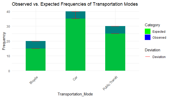
Chi-Square Goodness of Fit Test in R
Calculating Chi-square test on an airline dataset using chisq.test() function
In this example, we will use another method to calculate chi-square test in R. For this example, we will use an external dataset from the kaggle website.
Dataset Link: Flight Price Prediction
Make sure you replace the path of the file with the original path in your system.
R
data<- read.csv('path\to\your\file.csv')
cont_table <- table(data$airline, data$class)
chi_sq_result <- chisq.test(cont_table)
print(chi_sq_result)
|
Output:
Pearson's Chi-squared test
data: cont_table
X-squared = 60493, df = 5, p-value < 2.2e-16
We can also plot these values with the help of ggplot2 library in R
R
observed <- as.vector(cont_table)
expected <- chi_sq_result$expected
plot_data <- data.frame(
Category = rep(rownames(cont_table), 2),
Frequency = c(observed, expected),
Type = rep(c("Observed", "Expected"), each = nrow(cont_table))
)
library(ggplot2)
ggplot(plot_data, aes(x = Category, y = Frequency, fill = Type)) +
geom_bar(stat = "identity", position = position_dodge(width = 0.9), width = 0.7) +
labs(title = "Observed vs. Expected Frequencies",
y = "Frequency",
fill = "Type") +
theme_minimal() +
theme(axis.text.x = element_text(angle = 45, hjust = 1))
|
Output:
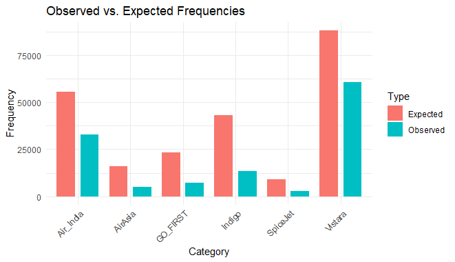
Chi-Square Goodness of Fit Test in R
As we saw our chi square test shows high discrepancy and our graph shows wide difference between the expected and observed frequencies too.
Calculating Chi-square test using vcd package
We can use ‘vcd’ package available in R to calculate the chi-square test and other statistical values that can help us understanding the dataset better. Here, we are creating a fictional dataset on different age groups of people using different brands of smart phones.
R
library(vcd)
set.seed(123)
age_groups <- c("Teenager", "Adult", "Senior")
smartphone_brands <- c("Samsung", "Apple", "Xiaomi", "Huawei", "Google")
n <- 1000
age_sample <- sample(age_groups, n, replace = TRUE)
smartphone_sample <- sample(smartphone_brands, n, replace = TRUE)
age_sample <- factor(age_sample, levels = age_groups)
smartphone_sample <- factor(smartphone_sample, levels = smartphone_brands)
cont_table <- table(age_sample, smartphone_sample)
chi_sq_result <- assocstats(cont_table)
print(chi_sq_result)
|
Output:
X^2 df P(> X^2)
Likelihood Ratio 10.856 8 0.20998
Pearson 10.961 8 0.20394
Phi-Coefficient : NA
Contingency Coeff.: 0.104
Cramer's V : 0.074
Calculating Chi-Square test using the prop.test() function
In this example we will create a fictional dataset of a drug test and use prop.test() function to get our values.
R
success_new_drug <- 45
failure_new_drug <- 15
success_standard_drug <- 30
failure_standard_drug <- 30
cont_table_2x2 <- matrix(c(success_new_drug, failure_new_drug, success_standard_drug,
failure_standard_drug), nrow = 2, byrow = TRUE)
chi_sq_result_2x2 <- prop.test(cont_table_2x2)
print(chi_sq_result_2x2)
|
Output:
2-sample test for equality of proportions with continuity correction
data: cont_table_2x2
X-squared = 6.9689, df = 1, p-value = 0.008294
alternative hypothesis: two.sided
95 percent confidence interval:
0.06596955 0.43403045
sample estimates:
prop 1 prop 2
0.75 0.50
We created a 2×2 contingency table where the rows represent treatment outcomes (success or failure) and the columns represent the two groups (new drug treatment vs. standard drug treatment).
We used the prop.test() function to perform a Chi-Square test for proportions on this 2×2 table.
Share your thoughts in the comments
Please Login to comment...