How to Perform a Likelihood Ratio Test in R

The Likelihood Ratio Test is a statistical method of testing the goodness of fit of two different nested statistical models using hypothesis testing. It is widely used in many industries for multiple reasons such as model comparison, hypothesis testing, variable selection, assessing model adequacy, and statistical inference in R Programming Language.

Likelihood Ratio Test

In statistics, the likelihood function represents the probability of observing the given data in a statistical model. This test compares two competing models, one is usually a simple model(null hypothesis) and the other is a more complex model(alternative hypothesis). The formula for the likelihood ratio test is given below:

Λ= -2log(L(restricted model)/L(full model))

where,

• L(restricted model): is the likelihood of the restricted model (null hypothesis).
• L(full model): is the likelihood of the full model (alternative hypothesis).
• Λ: is the likelihood ratio test statistic.

In simpler words, if we have two different models based on different numbers and sets of variables, let one be a simple model and another complex with more or other variables, the Likelihood Ratio tests if the variables make a significant change to consider in the results or not.

Performing likelihood ratio test for student performance prediction

In this example, we will create a fictional dataset on predicting student performance based on hours of study and participation in extracurricular activities. We’ll then fit two nested linear regression models to the data and perform a likelihood ratio test (LRT) to determine whether including the extracurricular activities variable significantly improves the model fit compared to a simpler model with only the intercept and hours of study as predictors.
Two important libraries that we will use here are

• ggplot2: ggplot2 library stands for grammar of graphics, popular because of its declarative syntax used to visualize and plot our data into graphs for better understanding.
• lmtest: This package in R programming language provides various statistical tests and diagnostic procedures for linear regression models.

We can divide calculating LRT into different steps and the code implementation is given below:

Step 1: Load Required Libraries

Firstly, we need to load and install the necessary packages for calculating LRT. To install new packages we can use the syntax: install.packages(“package name”)

R

library(ggplot2)
library(lmtest)

Output:

package ‘ggplot2’ was built under R version 4.3.2 

Loading required package: zoo

Attaching package: ‘zoo’

The following objects are masked from ‘package:base’:

    as.Date, as.Date.numeric

Step 2: Generate and Prepare Data

In this article, we are using a fictional dataset of students’ study hours, extracurricular activities, and student performance.

R

# Set seed for reproducibility
set.seed(123)

# Generate fictional data
hours_of_study <- rnorm(100, mean = 5, sd = 1.5)
extracurricular_activities <- rnorm(100, mean = 3, sd = 1)
student_performance <- 50 + 5 * hours_of_study + 3 * extracurricular_activities +
rnorm(100, mean = 0, sd = 5)

# Create a dataframe
data <- data.frame(hours_of_study, extracurricular_activities, student_performance)
head(data)

Output:

  hours_of_study extracurricular_activities student_performance
1       4.159287                   2.289593            88.65926
2       4.654734                   3.256884            89.60638
3       7.338062                   2.753308            93.62451
4       5.105763                   2.652457            86.20216
5       5.193932                   2.048381            80.04310
6       7.572597                   2.954972            94.34667

Step 3: Fit Models

Now, to perform Likelihood Ratio Test we need to fit models. Here we are using a Linear regression model to fit our data. lm() function is used to fit linear models. We will fit two models null and full model varying in the terms of variables used.

R

# Fit the null model (restricted)
null_model <- lm(student_performance ~ 1, data = data)

# Fit the full model (alternative)
full_model <- lm(student_performance ~ hours_of_study + extracurricular_activities,
                 data = data)

Step 4: Perform Likelihood Ratio Test

lrtest() function is used to perform the likelihood ratio test between the two models that we fit in the previous step.

R

# Perform likelihood ratio test
likelihood_ratio_test <- lrtest(null_model, full_model)
likelihood_ratio_test

Output:

Likelihood ratio test

Model 1: student_performance ~ 1
Model 2: student_performance ~ hours_of_study + extracurricular_activities
  #Df  LogLik Df  Chisq Pr(>Chisq)    
1   2 -352.60                         
2   4 -296.32  2 112.55  < 2.2e-16 ***
---
Signif. codes:  0 ‘***’ 0.001 ‘**’ 0.01 ‘*’ 0.05 ‘.’ 0.1 ‘ ’ 1

Model 1 : represents the null model, which includes only the intercept.

Model 2: represents the full model, which includes both hours_of_study and extracurricular_activities as predictors.

• #Df : This indicates the degree of freedom or the number of parameters involved
• LogLik: This indicates the log-likelihood values for each model.
• Chisq: is the likelihood ratio test statistic, which measures the difference in log-likelihood values between the two models.
• Pr(>Chisq): represents the p-value associated with the likelihood ratio test.

Step 5: Interpret Results

We can also write code to estimate and compare the results and find which model is better and if we should reject or accept our hypothesis,

R

# Interpretation of likelihood ratio test results
if (likelihood_ratio_test$"Pr(>Chisq)"[2] < 0.05)
{
  cat("Reject the null hypothesis. The full model is significantly better than
        the null model.\n")
} else {
  cat("Fail to reject the null hypothesis. The null model is sufficient.\n")
}

Output:

Reject the null hypothesis. The full model is significantly better than the null model.

Step 6: Additional Calculations

Some additional calculations like AIC or Akaike Information Criterion and Log-likelihood value are measured to compare the models.

R

# Calculate log-likelihood values
loglik_null <- logLik(null_model)
loglik_full <- logLik(full_model)

# Calculate AIC values
AIC_null <- AIC(null_model)
AIC_full <- AIC(full_model)

# Print log-likelihood values and AIC values
cat("Log-likelihood value (null model):", loglik_null, "\n")
cat("Log-likelihood value (full model):", loglik_full, "\n")
cat("AIC value (null model):", AIC_null, "\n")
cat("AIC value (full model):", AIC_full, "\n")

Output:

Log-likelihood value (null model): -352.5989 

Log-likelihood value (full model): -296.3219 

AIC value (null model): 709.1979 

AIC value (full model): 600.6438 

Log-likelihood values: A higher log-likelihood value indicates a better fit of the model to the data.

AIC values: AIC values stands for Akaike Information Criterion. It measures the relative quality of the given dataset of a statistical model. Lower AIC values indicate a better balance between goodness of fit and model complexity.

Step 7: Visualization

We can also plot these values to visualize and get a better understanding using the “ggplot2” package in the R programming Language.

R

# Plot the data
ggplot(data, aes(x = hours_of_study, y = student_performance)) +
  geom_point() +
  geom_smooth(method = "lm", se = FALSE, color = "blue") +
  labs(title = "Student Performance vs. Hours of Study",
       x = "Hours of Study",
       y = "Student Performance")

# Plot including extracurricular activities
ggplot(data, aes(x = extracurricular_activities, y = student_performance)) +
  geom_point() +
  geom_smooth(method = "lm", se = FALSE, color = "red") +
  labs(title = "Student Performance vs. Extracurricular Activities",
       x = "Extracurricular Activities",
       y = "Student Performance")

Output:

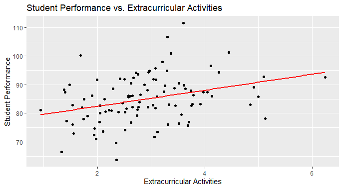
Perform a Likelihood Ratio Test in R

Performing LRT on a salary dataset

In this example, we will download a dataset from the Kaggle website based on the age, experience, and income of employees.
Dataset Link: Multiple Linear Regression Dataset

Make sure to replace the path of your file with the original path of the downloaded file in your system.

R

# Step 1: Load required libraries
library(lmtest)
library(ggplot2)

# Step 2: Load dataset
data <- read.csv('path\to\your\file.csv')

# Step 3: Fit the null model (restricted)
null_model <- lm(income ~ 1, data = data)

# Step 4: Fit the full model (alternative)
full_model <- lm(income ~ age + experience, data = data)

# Step 5: Calculate AIC values
AIC_null <- AIC(null_model)
AIC_full <- AIC(full_model)

# Step 6: Calculate log-likelihood values
loglik_null <- logLik(null_model)
loglik_full <- logLik(full_model)

# Step 7: Perform likelihood ratio test
lrt <- lrtest(null_model, full_model)
lrt

# Step 8: Comparison of AIC and log-likelihood values
cat("AIC value (null model):", AIC_null, "\n")
cat("AIC value (full model):", AIC_full, "\n")
cat("Log-likelihood value (null model):", loglik_null, "\n")
cat("Log-likelihood value (full model):", loglik_full, "\n")

# Step 9: Interpretation of likelihood ratio test results
if (lrt$"Pr(>Chisq)"[2] < 0.05) {
  cat("Reject the null hypothesis. The full model is significantly better than the null
        model.\n")
} else {
  cat("Fail to reject the null hypothesis. The null model is sufficient.\n")
}

Output:

Likelihood ratio test

Model 1: income ~ 1
Model 2: income ~ age + experience
  #Df  LogLik Df Chisq Pr(>Chisq)    
1   2 -208.68                        
2   4 -170.81  2 75.74  < 2.2e-16 ***
---
Signif. codes:  0 ‘***’ 0.001 ‘**’ 0.01 ‘*’ 0.05 ‘.’ 0.1 ‘ ’ 1

AIC value (null model): 421.3602 

AIC value (full model): 349.6206 

Log-likelihood value (null model): -208.6801 

Log-likelihood value (full model): -170.8103 

Reject the null hypothesis. The full model is significantly better than the null model.

We can also plot the values of this dataset for better visualization.

R

# Plot the data and fitted models
ggplot(data, aes(x = experience, y = income)) +
  geom_point() +
  geom_smooth(method = "lm", se = FALSE, color = "red") +
  labs(title = "Income vs. Experience",
       x = "Experience",
       y = "Income") +
  theme_minimal()

Output:

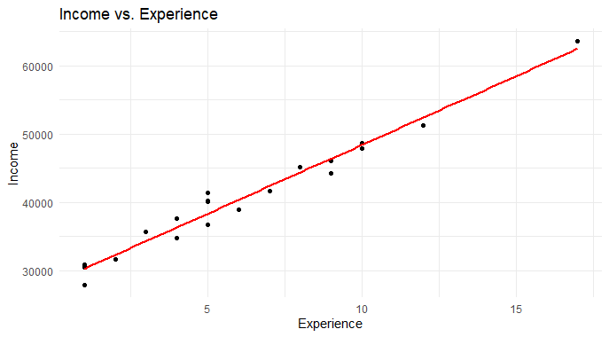
Perform a Likelihood Ratio Test in R

Conclusion

In this article, we understood how to calculate the Likelihood Ratio Test and its mathematical significance using R. We also plotted these values on the graph to understand in a better way.