Chi-Square Distribution in R

The chi-squared distribution with df degrees of freedom is the distribution computed over the sums of the squares of df independent standard normal random variables. This distribution is used for the categorical analysis of the data.

Let us consider X₁, X₂,…, X_m to be the m independent random variables with a standard normal distribution, then the quantity following the Chi-Squared distribution with m degrees of freedom can be evaluated as below. The mean of this distribution is m, and its variance is equivalent to 2*m, respectively.

Formula:

qchisq() function

qchisq gives the quantile function. When we supply the value of ncp = 0, the algorithm for the non-central distribution is used. The value of this method is equivalent to the value of x at the qth percentile (lower.tail = TRUE).

Syntax:

qchisq(p, df, ncp = 0, lower.tail = TRUE, log.p = FALSE)

Parameter : 

• p – vector of probabilities
• df – degrees of freedom 
• ncp – non-centrality parameter (non-negative).
• log.p – logical; if TRUE, probabilities p are given as log(p).
• lower.tail – logical; if TRUE (default), probabilities are P[X ≤ x], otherwise, P[X > x].

Example: 

R

# defining the degrees of freedom
free = 5
qchisq(.75, df=free)

Output

[1] 6.62568

This function can also be used to calculate quantile for a given area under the curve.

Example:

R

# defining the degrees of freedom
free = 5
qchisq(.999, df=free, lower.tail = TRUE)

Output

[1] 20.51501

dchisq() function

dchisq gives the density function. That is, it is used for computing the cumulative probability (lower.tail = TRUE for left tail, lower.tail = FALSE for right tail) of less than or equal to the value of vector of quantiles, that is q. 

Syntax:

dchisq(x, df, ncp = 0, log = FALSE)

Parameter :

• x – vector of quantiles
• df – degrees of freedom
• ncp – non-centrality parameter (non-negative).
• log.p – logical; if TRUE, probabilities p are given as log(p).

Example:

R

# defining degrees of freedom
df = 6
vec <- 1:4

print ("Density function values")

dchisq(vec, df = df)

Output

[1] “Density function values” 

[1] 0.03790817 0.09196986 0.12551072 0.13533528

pchisq() function

pchisq gives the distribution function.  dchisq(x, df) gives us the probability of χ2 with equivalent to a value of x when the degree of freedom is df. This method can be used to calculate the area under the curve for the specified intervals of the χ2-curve with a given number of degree of freedoms.

Syntax: 

pchisq(q, df, ncp = 0, lower.tail = TRUE, log.p = FALSE)

Parameter :

• q – vector of quantiles
• df – degrees of freedom
• ncp – non-centrality parameter (non-negative).
• log.p – logical; if TRUE, probabilities p are given as log(p).
• lower.tail – logical; if TRUE (default), probabilities are P[X ≤ x], otherwise, P[X > x].

Example:

R

# defining degrees of freedom
df = 5

# calculating for the values in the interval [0,5]
print ("Calculating for the values [0,5]")
pchisq(5, df = df,lower.tail = TRUE)

# calculating for the values in the interval [5,inf)
print ("Calculating for the values [5,inf)")
pchisq(5, df = df,lower.tail = FALSE)

Output

[1] “Calculating for the values [0,5]” 

[1] 0.5841198 

[1] “Calculating for the values [5,inf)” 

[1] 0.4158802

The summation of the curves under both the intervals [0,5] and [5,∞) is equivalent to 1.

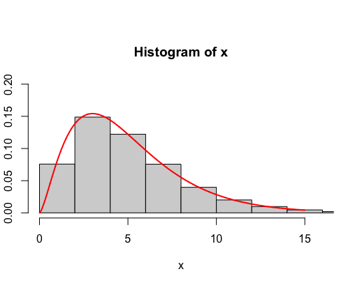
rchisq() function

rchisq(n, df) returns n random numbers from the chi-square distribution. It is therefore to generate random deviates. 

Syntax:

rchisq(n, df, ncp = 0)

Parameter : 

• n – number of observations. If length(n) > 1, the length is taken to be the number required.
• df – degrees of freedom (non-negative, but can be non-integer).
• ncp – non-centrality parameter (non-negative).

Example:

R

# computing values of 50k random values with 5 degrees of freedom
x <- rchisq(50000, df = 5)

hist(x,
     freq = FALSE,
     xlim = c(0,16),
     ylim = c(0,0.2))

curve(dchisq(x, df = 5), from = 0, to = 15,
      n = 5000, col= 'red', lwd=2, add = T)

Output