Spreadsheets are grid-based files containing scalable entries that are used to organize data and make calculations. Spreadsheets are used by people all around the world to build tables for personal and corporate purposes. You may also utilize the tool to make sense of your data by using its features and formulas. You could, for example, use a spreadsheet to track data and see sum, difference, multiplication, division, fill date automatically, etc.
Rows & Columns in Excel Spreadsheets
In Excel, rows and columns are two different properties that combine to form a cell, a range, or a table. In general, the vertical portion of an Excel worksheet is known as columns, and there can be 256 of them in a worksheet, while the horizontal portion is known as rows, and there can be 1048576 of them.
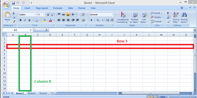
Here, we can see Row 3 highlighted with red color & Column B highlighted with green color. Every row has 256 columns & every column has 1048576 rows.
Cell Referencing
A cell reference, also known as a cell address, is a technique that combines a column letter and a row number to describe a cell on a worksheet. Using cell references, we can refer to any cell on the worksheet (in Excel formulas).
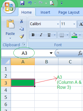
Here we refer to the cell in column A & row 3 by :A3. You can make use of such notations in any of the formulae or copy the value of one cell to another cell (by using = A3)
Enter Numbers, Text, Date/time, Series Using AutoFill
You can go to a particular cell & enter the data in that cell. The data can be of the type date, numeric, text, etc.
Step 1. Go to the cell where you want to enter the data
Step 2. Click on that cell
Step 3. Enter the required data.
(a) Excel Date Type
In an Excel cell, you can input a date in a variety of ways, such as 11/06/2021, 11-Jun-2021, or 11-Jun, or June 11, 2021. When you input this in a cell, Microsoft Excel recognizes that you’re entering a date and applies date format to that cell automatically. Excel usually prepares the newly inserted date according to the default date settings in Windows, but it can also leave it exactly as you typed.
In the given example: B2 contains Number, A2 & A4 contains Text & B4 contains date.
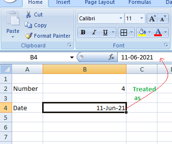
Note: Left – Justify the date in case any problem arises.
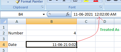
(b) Insert Time Stamp
You can enter the time along with the date as 11-06-2021 0:12 as shown below:
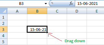
(c) Auto fill a date that increases in the series 1 by 1 day
Step 1: Enter a start date in the starting cell
Step 2: To add dates to cells, pick the cell with the first date and drag the fill handle across or down the cells where you want Excel to add dates. (When you pick a cell or a range of cells in Excel, the fill handle displays as a small green square in the bottom-right corner, as illustrated in the screenshot below.)
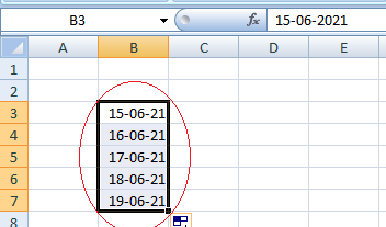
Your dates are filled Up automatically till the cell, up to which you dragged down. You can see the consecutive dates in column B have a difference of 1 day.
Edit and Format a Worksheet
You can do a lot of editing & formatting in a worksheet, like:
(a) Changing the Color:
Step 1: Select the cell(s) for whose data you want to change the color
Step 2: From the formatting toolbar above, choose the font color & click on that color.
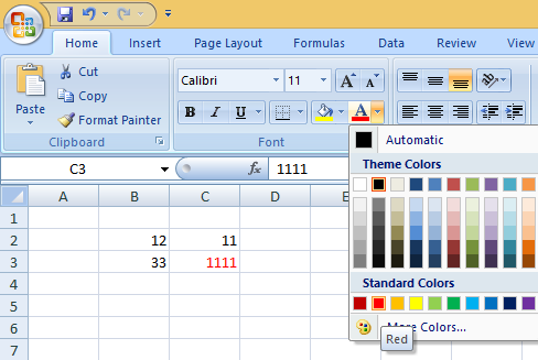
The color will be applied(Like C3 here has its data in the color red)
(b) Changing the Font Style:
Step 1: Select the cell(s) for whose data you want to change the font style
Step 2: From the formatting toolbar above, choose the font style & choose any one style & click on it.
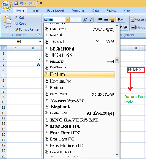
Like, in the above example we opt for the font style: “Dotum” for cell H4
(c) Alignment of Text:
The appearance and direction of the paragraph’s edges are determined by alignment. Types of alignment are:
- Left Alignment: The text was aligned uniformly along the left margins.
- Right Alignment: The text was aligned uniformly along the right margins.
- Center Alignment: The text is aligned evenly with the center of the page.
Steps to apply any 1 alignment on cell(s):
Step 1: Select the cell(s) for whose data you want to change the font Alignment.
Step 2: From the formatting toolbar above, choose the alignment type & click on it.
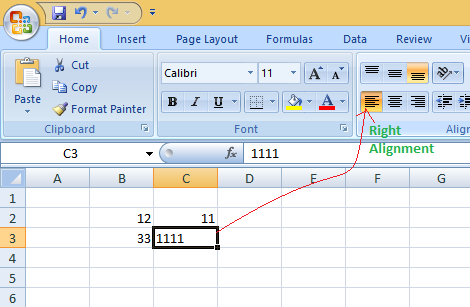
Like, in the above example we opt for the Right Alignment for cell C3.
Insert and Delete Cells
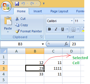
(a) Inserting a Cell
To insert a cell in between 2 cells follow these steps:
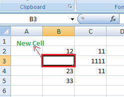
Say, for example we want to insert a cell between B2 & B3, then:
Step 1: Select the cell above which you want to insert(say B3 here)
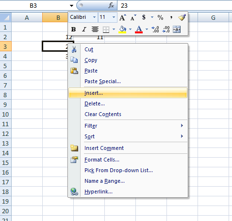
Step 2: Right-click the cell, a menu will pop up. Click on insert under it.
Step 3: A window for insert will pop up. To insert a new cell: (a) above the selected cell, choose shift cells down
(b) left to the selected cell, choose shift cells right
(Note: To insert a complete row upward/a column to the left, choose an option, entire row & entire column)
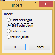
Step 4: Click Ok. A new cell will be inserted
Like, in the above example we opt for the font style: “Dotum” for cell H4
(b) Deleting a cell
To delete a cell follow the following steps:
Say, for example, we want to delete a cell B3, then:
Step 1: Select the cell for deletion(say B3 here)
Step 2: Right-click the cell, a menu will pop up. Click on delete under it.
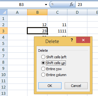
Step 3: A window for delete will pop up. To delete cell & move: (a) Shifts cells below it upward, choose shift cells up (b) Shift cells after it to the left, choose shift cells left
(Note: To delete a complete row/a column, choose option, entire row & entire column)
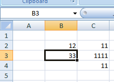
The cell will be deleted.
Formula Using the Arithmetic Operators
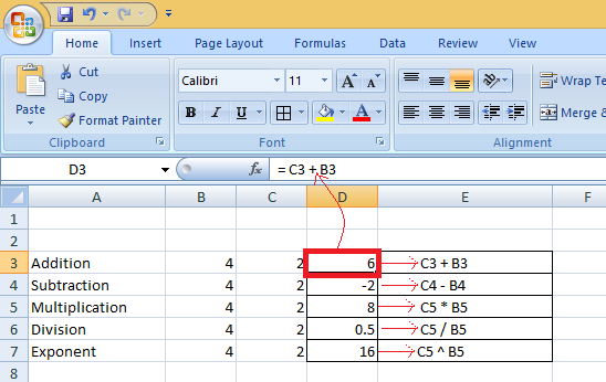
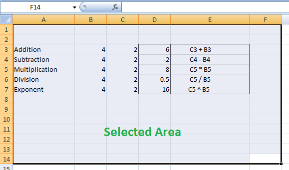
For formulas, Excel utilizes common operators such as the plus symbol (+), the minus sign (-), an asterisk for multiplication (*), a forward slash for division (/), and a caret () for exponents.
| Operation |
Symbol |
| Addition |
+ |
| Multiplication |
* |
| Division |
/ |
| Subtraction |
– |
| Exponent |
^ |
In the given example, we calculate:
- Sum: C3 + B3 = 4 + 2 = 6
- Subtraction: C4 – B4 = 2 -4 = -2
- Multiplication: C5 * B5 = 2 * 4 = 8
- Division: C5 / B5 = 2/4 = 0.5
- Exponent: C5 ^ B5 = 2^4 = 16
Print a Worksheet using the attached printer
Step 1: Select the area of the spreadsheet you want to print.
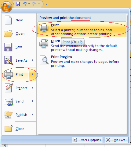
Step 2: Click on the Microsoft icon
Step 3: Click On Print & a window for Print & Preview the document will pop up.
Step 4: Click on Print. Then a window for Print will pop up.
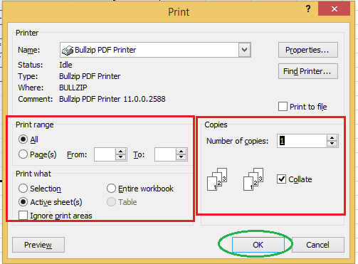
Step 5: Select the printer by which you want to take out a print of the document. Select the page range (Print of all or some or current page) & the number of copies you want.
Step 6: Click on OK. You will get a print of your selected area of the Spreadsheet.
Note: Shortcut for print is Ctrl + p.
Sample Questions
Question 1. To enter the current date & time, what are the shortcuts?
Answer:
(i) Ctrl +; – To insert current date (or use Today() function)
(ii) Ctrl + Shift + ; – To insert the current time. (or use Now() function)|
(iii) Ctrl + ; & then Space key & then Ctrl + Shift + ; – To enter both current date & time
Question 2. Define active & inactive cell in spreadsheets.
Answer:
Active Cell: The cell on which you clicked & has a dark color boundary is active cell.
Inactive Cells: The cell which is not active is called inactive cell(Remaining cells except active one).
Question 3. How can the dates be interpreted in Excel?
Answer:
Dates are interpreted in Excel as
(a) dd-mm-yyyy
(b) dd-mm-yy
(c) dd/mm/yy
(d) yyyy-mm-dd
(e) dd mmm yyyy
Question 4. What kind of data can be entered in the cells?
Answer:
The data in the cell can be under the 4 categories: text, values, formulas & dates.
Question 5. What should you do if you wish to change an existing cell entry?
Answer:
To edit an existing cell entry:
(a) Select the cell and press the F2 key
(b) Then move the pointer to the needed location
(c) make the necessary changes
(d) Last but not least, press the Enter key.
Share your thoughts in the comments
Please Login to comment...