Word Embedding in Pytorch

Word Embedding is a powerful concept that helps in solving most of the natural language processing problems. As the machine doesn’t understand raw text, we need to transform that into numerical data to perform various operations. The most basic approach is to assign words/ letters a vector that is unique to them but this approach is not very useful as the words with similar meanings will get completely different vectors. Another more useful approach is training a model that can generate vectors of words. This is better than the previous approach because it will group similar words together and generate similar vectors for them. It also captures the overall meaning/ context of the words and sentences which is better than random assignment of vectors.

Embedding

Embeddings are real-valued dense vectors (multi-dimensional arrays) that carry the meaning of the words. They can capture the context of the word/sentence in a document, semantic similarity, relation with other words/sentences, etc. A popular example of how they extract the contexts from the words is if you remove a man from the king and add a woman, it will output a vector similar to a queen. Also, similar words are close to each other in the embedding space. Many pre-trained models are available such as Word2Vec, GloVe, Bert, etc.

Pytorch Embedding

As defined in the official Pytorch Documentation, an Embedding layer is – “A simple lookup table that stores embeddings of a fixed dictionary and size.” So basically at the low level, the Embedding layer is just a lookup table that maps an index value to a weight matrix of some dimension. This weight matrix is further optimised during training (updated during backpropagation to reduce the loss) to produce more useful vectors.

Working

Now let’s look into the working of embedding in Pytorch. When an embedding layer is created, an embedding matrix is initialised with random vectors having dimensions of (num_embeddings, embedding_dim). This is basically our lookup table where our words are mapped to indexes.

Given an input word or token, represented by its index in the vocabulary, you pass this index to the embedding layer which then looks up the corresponding row in the embedding matrix. The embedding vector is then extracted from the row as output which is of the dimension embedding_dim.

During training, the embedding vectors are updated through backpropagation to minimize the loss. This means the vectors are adjusted to better represent the semantics and relationships between words.

Embedding layer takes minimum of two arguments – num_embeddings and embedding_dim. There are various other optional parameters also such as padding_idx, max_norm, etc. Refer to the official docs for this. Now the first required parameter is num_embeddings which means what is the dictionary size. For example, if you have a vocabulary of 5000 words, then the value that will go into the first parameter will be 5000. The second required parameter is embedding_dim which means the size of each embedding vector(as all the learned vectors will have a fixed size).

CBOW and Skip-gram Techniques

There are two major techniques in embeddings known as Continuous Bag of Words (CBOW) and Skip gram. Let’s learn about them a little below-

Continuous Bag of Words (CBOW)– BOW predicts a target word based on the surrounding context words. This means that, for it to predict the focus word (the word we are interested in), it checks the surrounding words around it. The contextual representation of surrounding words for the focus word, helps in clearly predicting the word. It takes a pre-defined fixed window size into account and tries to predict the target word.

Example- Suppose we have a sentence – “I eat pizza every day”. So, if we have a context window of 2, the input will be [“I”, “pizza”] and the target will be “eat”.

CBOW

In the above diagram, W(t-2) and W(t-1) represent the words before our focus word, i.e., [‘I’, ‘eat’]. And W(t+1), W(t+2) represent the words after focus word, i.e., [‘every’, ‘day’]. These four words are used to predict the focus word, that is, “pizza”. So when given the task to get embedding for each word in the vocabulary by following Continuous Bag of Words, the context_window is taken as 2, the (context_words, focus word) pairs would be:

([‘I’, ‘pizza’], ‘eat’), ([‘eat’, ‘every’], ‘pizza’), ([‘pizza’, ‘day’], ‘every’).

(Note: You can choose the context window of your own choice)

Skip-gram– Skip gram technique is similar to the continuous bag of words but the main difference is instead of predicting the target word from the context, this takes the target word as input and tries to predict the context (which is a set of words). Example- If we take the above sentence, the input will be “eat” and the target will be [“I”, “pizza”].

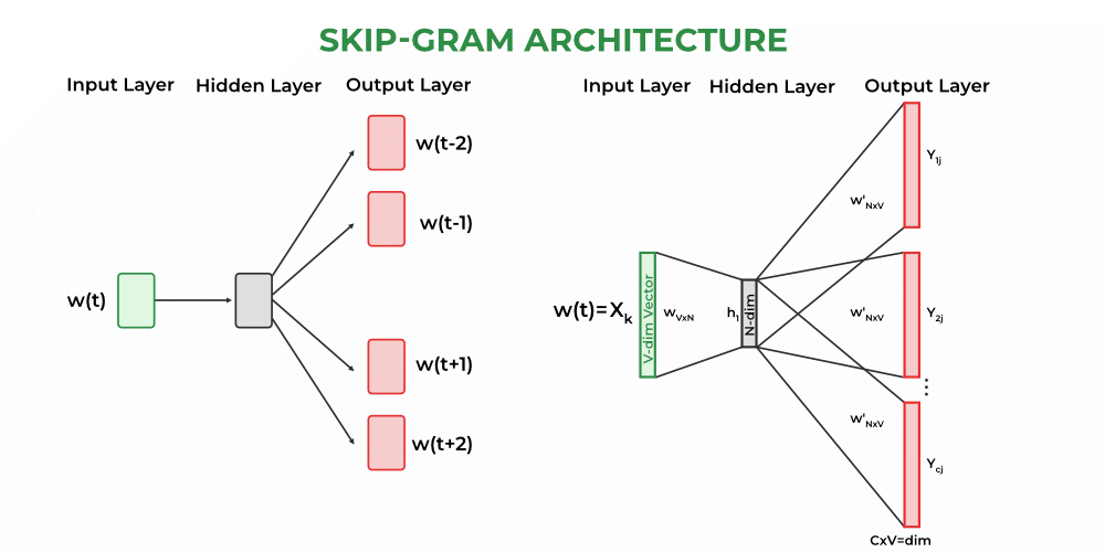
Skip-gram

Here, the context words for the focus word is predicted. As seen from the diagram above, for each input word the neighbouring context words will be predicted. To get multiple outputs from a single input, a SoftMax activation is used to assign probability for the context words. We will consider the same context window of 1 and see how the (context word, focus words) look like:

(‘eat’, [‘I’, ‘pizza’]), (‘pizza’, [‘eat’, ‘every’]), (‘every’, [‘pizza’, ‘day’])

Model Building in Pytorch

Before we dive into the modelling building, lets first understand how the Embedding layer syntax works in Pytorch. It is give as:

torch.nn.Embedding(num_embeddings,
 embedding_dim,
 padding_idx=None,
 max_norm=None,
 norm_type=2.0,
 scale_grad_by_freq=False,
 sparse=False)

where,

1. num_embeddings (int) is the size of the vocabulary
2. embedding_dim (int) talks about size of each embedding vector
3. padding_idx(int, optional) is used to treat a specific index as padding token
4. max_norm (float, optional) limits the normalisation to a specific value, thus, avoiding exploding gradient.
5. norm_type (float, optional) specifies the type of normalisation (L1 or L2)
6. scale_grad_by_freq(bool, optional) scales the embeddings based on the frequency of the words in the vocab.
7. sparse (bool, optional) decides whether to use sparse gradient updates for getting embedding gradients, when it is set to True

Now let’s look at some code to see how this works.

Example 1:

Firstly, we’ll import all the libraries required.

Python

import torch
import torch.nn as nn

# Embedding layer with 5 vocab size and 40 vector embeddings.
embedding = nn.Embedding(5, 40)
#passing the input
embed = embedding(torch.LongTensor([1]))
#print embeddings
print(embed)

Output:

tensor([[ 2.5257,  1.0342, -0.3173, -0.6847,  1.1305, -1.1096, -1.1943, -0.7296,
         -0.3663,  0.0923, -0.4928,  0.6728,  0.3144, -0.1297, -0.4178,  0.5037,
          1.0004, -0.2568,  0.0439, -0.0526, -0.4425, -0.8101, -1.4096,  0.3209,
         -0.4986, -0.2673, -0.5162, -0.7360, -0.3854,  0.4884,  1.0126, -0.5779,
         -0.4810, -0.1298, -0.4205, -0.6634,  0.5938,  1.9682,  0.1999,  1.2953]],
       grad_fn=<EmbeddingBackward0>)
torch.Size([1, 40])

The above code basically created a lookup table named embedding which has 5 rows and 40 columns. Each row will represents a single word embedding initialized randomly between -1 and 1.

You can also see the shape of the vector printed at the end. It’s the same as we defined in our parameter. These vectors later gets optimised during training to make more meaningful vectors. Now let’s look at an example that’s present in the docs.

Code:

Firstly, we’ll import all the required libraries. For this, we’ll be needing torch and the nn module from torch. Then we’ll set the manual seed to 1 to control the randomness.

Python

import torch
import torch.nn as nn

torch.manual_seed(1)

Then, we’ll create a dictionary which has the numerical mappings of the words and initialise the embedding layer by using nn.Embedding of shape (2,5).

Python

#creating the dictionary
word_to_ix = {"geeks": 0, "for": 1, "code":2}
#creating embedding layer - 3 words in vocab, 5-dimensional embeddings
embeds = nn.Embedding(2, 5)

Then the next step is to convert the numerical mapping of the word (which we want to create embedding for) into tensor with the dtype long. We use LongTensors as they can be used to represent labels/categories. We can access the embeddings of the word “geeks” as shown below using the embeds.

Python

#converting to tensor
lookup_tensor = torch.tensor([word_to_ix["geeks"]], dtype=torch.long)
#accessing the embeddings of the word "geeks"
pytorch_embed = embeds(lookup_tensor)

Finally, we’ll print the embeddings.

Python

#print the embeddings
print(pytorch_embed)

Output:

tensor([[ 0.6614,  0.2669,  0.0617,  0.6213, -0.4519]],
       grad_fn=<EmbeddingBackward0>)

As these are randomly initialised vectors so they are not of much significance. They can be optimised through training but that will require a lot of effort. To show case how other padding affect an embedding, let’s take a look at another example.

Example 2:

We will take a dummy sentence and using Counter, create a dictionary of words with keys as the words and their frequency as the value.

Python3

from collections import Counter

# This is going to be the dummy sentence :
sentences = "this is the second example showing for the article at gfg. and doing this is actually really fun"

words = sentences.split(' ')

# create a dictionary
vocab = Counter(words)
vocab = sorted(vocab, key=vocab.get, reverse=True)
vocab_size = len(vocab)

# create a word to index dictionary from our Vocab dictionary
word2idx = {word: ind for ind, word in enumerate(vocab)}

encoded_sentences = [word2idx[word] for word in words]

# assign a value to your embedding_dim
e_dim = 5

After creating the dictionary and assigning a value for our embedding dimension, we are ready to initialise the embedding and see its output, but this time we are going to introduce padding index at position 4. What this will do is, pad the input at the specific index and assign a value of zero there.

Python3

# initialise an Embedding layer from Torch
emb = nn.Embedding(vocab_size, e_dim, padding_idx = 3)
word_vectors = emb(torch.LongTensor(encoded_sentences))

#print the word_vectors
print(word_vectors)

Output:

tensor([[-0.6125,  2.1841, -0.5777, -0.4984, -1.1440],
        [-0.2335, -0.4090,  0.9648, -0.4256,  0.8362],
        [ 1.1355,  0.1626,  2.7858,  0.2537, -1.0708],
        [ 0.0000,  0.0000,  0.0000,  0.0000,  0.0000],
        [-0.1541,  0.9336,  0.5681,  0.2360,  0.2519],
        [-1.1530,  0.6917, -1.9961, -0.6608,  0.4884],
        [ 1.8149,  1.0138,  1.4318, -0.3035,  1.3098],
        [ 1.1355,  0.1626,  2.7858,  0.2537, -1.0708],
        [-1.1981,  2.6248, -0.4739, -0.6791, -0.0200],
        [ 0.8023,  1.0044, -0.9132, -0.0626, -0.7896],
        [-1.1518, -0.6600,  1.0331,  0.9817,  0.0572],
        [-0.7707, -1.9172,  0.1438, -0.3755, -0.4840],
        [-1.4134, -0.1180,  1.7339,  2.1844, -1.2160],
        [-0.6125,  2.1841, -0.5777, -0.4984, -1.1440],
        [-0.2335, -0.4090,  0.9648, -0.4256,  0.8362],
        [-0.6005, -0.7831,  1.0127,  1.6974, -1.9878],
        [-0.7868, -0.7832,  0.8435, -0.8540, -0.2374],
        [-1.8418,  0.3408, -1.8767,  1.2411,  1.2132]],
       grad_fn=<EmbeddingBackward0>)

As you can see, the embedding layer provided for the sentences contains padded values at index 3.

(Note: Embedding layer has one trainable parameter called weights, which is by default set to True. When using a pre-trained embedding, this can be set to False using “emb.weight.requires_grad = False“, but its implementation is beyond the scope of this article.)

Other than this, nn.Embedding layer is a key component in transformer architecture. In transformers, it is used to convert input tokens into continuous representations. In conclusion, the nn.Embedding layer is a fundamental component in many NLP models. Understanding this layer and how it works is an important step in building natural language processing models with pytorch effectively.