Locally Linear Embedding in machine learning

LLE(Locally Linear Embedding) is an unsupervised approach designed to transform data from its original high-dimensional space into a lower-dimensional representation, all while striving to retain the essential geometric characteristics of the underlying non-linear feature structure. LLE operates in several key steps:

• Firstly, it constructs a nearest neighbors graph to capture these local relationships. Then, it optimizes weight values for each data point, aiming to minimize the reconstruction error when expressing a point as a linear combination of its neighbors. This weight matrix reflects the strength of connections between points.
• Next, LLE computes a lower dimensional representation of the data by finding eigenvectors of a matrix derived from the weight matrix. These eigenvectors represent the most relevant directions in the reduced space. Users can specify the desired dimensionality for the output space, and LLE selects the top eigenvectors accordingly.

As an illustration, consider a Swiss roll dataset, which is inherently non-linear in its high-dimensional space. LLE, in this case, works to project this complex structure onto a lower-dimensional plane, preserving its distinctive geometric properties throughout the transformation process.”

Mathematical Implementation of LLE Algorithm

The key idea of LLE is that locally, in the vicinity of each data point, the data lies approximately on a linear subspace. LLE attempts to unfold or unroll the data while preserving these local linear relationships.

Here is a mathematical overview of the LLE algorithm:

Minimize:

Subject to :

Where:

• x_i represents the i-th data point.
• w_ij are the weights that minimize the reconstruction error for data point x_i using its neighbors.

It aims to find a lower-dimensional representation of data while preserving local relationships. The mathematical expression for LLE involves minimizing the reconstruction error of each data point by expressing it as a weighted sum of its k nearest neighbors‘ contributions. This optimization is subject to constraints ensuring that the weights sum to 1 for each data point. Locally Linear Embedding (LLE) is a dimensionality reduction technique used in machine learning and data analysis. It focuses on preserving local relationships between data points when mapping high-dimensional data to a lower-dimensional space. Here, we will explain the LLE algorithm and its parameters.

Locally Linear Embedding Algorithm

The LLE algorithm can be broken down into several steps:

• Neighborhood Selection: For each data point in the high-dimensional space, LLE identifies its k-nearest neighbors. This step is crucial because LLE assumes that each data point can be well approximated by a linear combination of its neighbors.
• Weight Matrix Construction: LLE computes a set of weights for each data point to express it as a linear combination of its neighbors. These weights are determined in such a way that the reconstruction error is minimized. Linear regression is often used to find these weights.
• Global Structure Preservation: After constructing the weight matrix, LLE aims to find a lower-dimensional representation of the data that best preserves the local linear relationships. It does this by seeking a set of coordinates in the lower-dimensional space for each data point that minimizes a cost function. This cost function evaluates how well each data point can be represented by its neighbors.
• Output Embedding: Once the optimization process is complete, LLE provides the final lower-dimensional representation of the data. This representation captures the essential structure of the data while reducing its dimensionality.

Parameters in LLE Algorithm

LLE has a few parameters that influence its behavior:

• k (Number of Neighbors): This parameter determines how many nearest neighbors are considered when constructing the weight matrix. A larger k captures more global relationships but may introduce noise. A smaller k focuses on local relationships but can be sensitive to outliers. Selecting an appropriate value for k is essential for the algorithm’s success.
• Dimensionality of Output Space: You can specify the dimensionality of the lower-dimensional space to which the data will be mapped. This is often chosen based on the problem’s requirements and the trade-off between computational complexity and information preservation.
• Distance Metric: LLE relies on a distance metric to define the proximity between data points. Common choices include Euclidean distance, Manhattan distance, or custom-defined distance functions. The choice of distance metric can impact the results.
• Regularization (Optional): In some cases, regularization terms are added to the cost function to prevent overfitting. Regularization can be useful when dealing with noisy data or when the number of neighbors is high.
• Optimization Algorithm (Optional): LLE often uses optimization techniques like Singular Value Decomposition (SVD) or eigenvector methods to find the lower-dimensional representation. These optimization methods may have their own parameters that can be adjusted.

LLE (Locally Linear Embedding) represents a significant advancement in structural analysis, surpassing traditional density modeling techniques like local PCA or mixtures of factor analyzers. The limitation of density models lies in their inability to consistently establish a set of global coordinates capable of embedding observations across the entire structural manifold. Consequently, they prove inadequate for tasks such as generating low-dimensional projections of the original dataset. These models excel only in identifying linear features, as depicted in the image below. However, they fall short in capturing intricate curved patterns, a capability inherent to LLE.

Enhanced Computational Efficiency with LLE. LLE offers superior computational efficiency due to its sparse matrix handling, outperforming other algorithms.

Implementation of Locally Linear Embedding

Importing Libraries

Python3

#importing Libraries
import numpy as np
import matplotlib.pyplot as plt
from sklearn.datasets import make_swiss_roll
from sklearn.manifold import LocallyLinearEmbedding

The code starts by importing necessary libraries, including numpy, matplotlib.pyplot, make_swiss_roll from sklearn.datasets, and LocallyLinearEmbedding from sklearn.manifold.

Generating a Synthetic Dataset (Swiss Roll)

Python3

# Code for Generating a synthetic dataset (Swiss Roll)
n_samples = 1000
# Define the number of neighbors for LLE
n_neighbors = 10
X, _ = make_swiss_roll(n_samples=n_samples)

It generates a synthetic dataset resembling a Swiss Roll using the make_swiss_roll function from scikit-learn.

n_samples specifies the number of data points to generate.
n_neighbors defines the number of neighbors used in the LLE algorithm.

Applying Locally Linear Embedding (LLE)

Python3

# Including Locally Linear Embedding
lle = LocallyLinearEmbedding(n_neighbors=n_neighbors, n_components=2)
X_reduced = lle.fit_transform(X)

An instance of the LLE algorithm is created with LocallyLinearEmbedding. The n_neighbors parameter determines the number of neighbors to consider during the embedding process.

The LLE algorithm is then fitted to the original data X using the fit_transform method. This step reduces the dataset to two dimensions (n_components=2).

Visualizing the Original and Reduced Data

Python3

# Code for Visualizing the original Versus reduced data
plt.figure(figsize=(12, 6))

plt.subplot(121)
plt.scatter(X[:, 0], X[:, 1], c=X[:, 2], cmap=plt.cm.Spectral)
plt.title("Original Data")
plt.xlabel("Feature 1")
plt.ylabel("Feature 2")

plt.subplot(122)
plt.scatter(X_reduced[:, 0], X_reduced[:, 1], c=X[:, 2], cmap=plt.cm.Spectral)
plt.title("Reduced Data (LLE)")
plt.xlabel("Component 1")
plt.ylabel("Component 2")

plt.tight_layout()
plt.show()

Output:

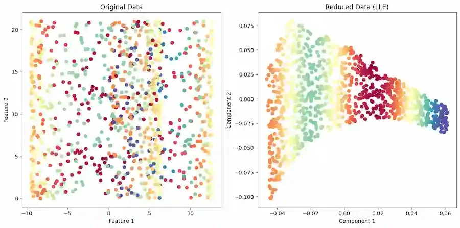
Locally Linear Embedding

In the second subplot , the reduced data obtained from LLE (X_reduced) is visualized in a similar manner to the original data. The color of the data points is still determined by the third feature of the original data (X[:, 2]).The plt.tight_layout() function is used to ensure proper spacing between subplots.

Advantages of LLE

The dimensionality reduction method known as locally linear embedding (LLE) has many benefits for data processing and visualization. The following are LLE’s main benefits:

• Preservation of Local Structures: LLE is excellent at maintaining the in-data local relationships or structures. It successfully captures the inherent geometry of nonlinear manifolds by maintaining pairwise distances between nearby data points.
• Handling Non-Linearity: LLE has the ability to capture nonlinear patterns and structures in the data, in contrast to linear techniques like Principal Component Analysis (PCA). When working with complicated, curved, or twisted datasets, it is especially helpful.
• Dimensionality Reduction: LLE lowers the dimensionality of the data while preserving its fundamental properties. Particularly when working with high-dimensional datasets, this reduction makes data presentation, exploration, and analysis simpler.

Disavantages of LLE

• Curse of Dimensionality: LLE can experience the “curse of dimensionality” when used with extremely high-dimensional data, just like many other dimensionality reduction approaches. The number of neighbors required to capture local interactions rises as dimensionality does, potentially increasing the computational cost of the approach.
• Memory and computational Requirements: For big datasets, creating a weighted adjacency matrix as part of LLE might be memory-intensive. The eigenvalue decomposition stage can also be computationally taxing for big datasets.
• Outliers and Noisy data: LLE is susceptible to anomalies and jittery data points. The quality of the embedding may be affected and the local linear relationships may be distorted by outliers.