How to use Box Cox transformation in the caret package in R?

In this article, we will see how to use a Box Cox Transformation in R Programming Language using the caret package.

Box Cox Transformation in R

The Box Cox Transformation in R is the technique used to transform non-normal data to a normal distribution by applying the power transformation. This transformation is commonly used in statistical modeling to improve the normality of the data and to stabilize the variance. The caret package in R provides a convenient way to apply Box Cox transformation to predictor variables in a dataset.

The following equation defines the Box Cox Transformation in R:

y(lambda) = (y^lambda - 1) / lambda, if lambda != 0
log(y), if lambda = 0

λ	Transformation
-2	1/x^2
-1	1/x
-0.5	1/sqrt(x)
0	log(x)
0.5	sqrt(x)
1	x
2	x^2

where y is the original variable, lambda is the transformation parameter, and y(lambda) is the transformed variable.

The box cox function in R

We will use MASS package and find out the Box Cox transformation in R.

R

library(MASS)

# Create data
y <- c(10, 10, 20, 25, 28, 30, 35, 38, 60, 70, 80)
x <- c(70, 75, 80, 35, 25, 40, 45, 60, 65, 70, 55)

# Find optimal lambda for Box-Cox transformation
bc <- boxcox(y ~ x)
lambda <- bc$x[which.max(bc$y)]

Output:

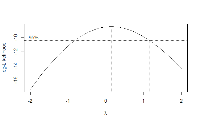
Box Cox transformation in R

We create two vector and then we apply Box Cox to Find optimal lambda for Box Cox Transformation in R.

Transform response variable using Box Cox

R

# Transform response variable using Box-Cox
y_transformed <- ((y^lambda - 1) / lambda)

# Print the results
cat("Original Data:\n")
print(data.frame(y, x))

cat("\nOptimal lambda for Box-Cox Transformation:", lambda, "\n")

cat("\nTransformed Data:\n")
print(data.frame(y_transformed, x))

Output:

Original Data:
    y  x
1  10 70
2  10 75
3  20 80
4  25 35
5  28 25
6  30 40
7  35 45
8  38 60
9  60 65
10 70 70
11 80 55

Optimal lambda for Box-Cox Transformation: 0.1414141 

Transformed Data:

   y_transformed  x
1       2.721696 70
2       2.721696 75
3       3.730249 80
4       4.076538 35
5       4.256637 25
6       4.367701 40
7       4.619802 45
8       4.756560 60
9       5.545769 65
10      5.823832 70
11      6.069650 55

Box Cox transformation using caret package in R

Now we will perform Box Cox transformation in the caret package in R Programming Language.

Caret Package 

The caret package in R (short for Classification And Regression Training) is a powerful toolkit for building and evaluating predictive models. It provides a unified interface to a wide variety of machine learning algorithms and data preprocessing techniques, making it easy to experiment with different models and techniques in a consistent and reproducible way.

Steps to use Box Cox Transformation in R

Step 1: Load the packages

First of all, we will load the required packages, that is, the caret package to apply Box Cox transformation and the ggplot2 package for a graphical representation of the data.

library(caret)
library(ggplot2)

Step 2: Load the dataset

Then load the dataset. We may either use R’s inbuilt dataset or we can create our own dataset. We may use various functions like rlnorm() or rgamma() to define our dataset.

data <- rgamma(...)

Step 3: Apply Box Cox transformation

Apply the Box Cox transformation using the BoxCoxTrans() function and pass the dataset as the parameters.

bc_trans <- BoxCoxTrans(data)

Step 4: Predict the value

transformed_data <- predict(bc_trans, data)

Step 5: Plot the model

The last step will be to plot the histogram after the transformation.

ggplot(data.frame(x = transformed_data), aes(x)) +
  geom_histogram(binwidth = 0.8, color = "black", fill = "lightblue") +
  ggtitle("Histogram of Box-Cox Transformed Data")

Transforming Non-Normal Data using Box Cox Transformation in R

To use the Box-Cox transformation in caret, we can use the BoxCoxTrans() function add pass the dataset to it. We will perform the BoxCox transformation on two types of data, namely the positively skewed data and negatively skewed data. Let us see the example for the same.

Positively Skewed Data

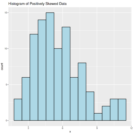
Positive Skewed data means the tail on the right side of the distribution is longer. The mean and median will be greater than the mode. Let us apply the BoxCox transformation to the positively skewed data.

In this example, we will generate a histogram of positively skewed data and then performs a Box Cox transformation on the data using the caret package in R. The transformed data is then plotted as a histogram.

R

# load the libraries
library(caret)
library(ggplot2)

# define skewed data
set.seed(124)
data <- rgamma(100, shape = 6, scale = 1)

# plot histogram of the skewed data
ggplot(data.frame(x = data), aes(x)) +
  geom_histogram(binwidth = 0.7, color = "black", fill = "lightblue") +
  ggtitle("Histogram of Positively Skewed Data")

# Box-Cox transformation using caret package
bc_trans <- BoxCoxTrans(data)
transformed_data <- predict(bc_trans, data)

# plot histogram of transformed data
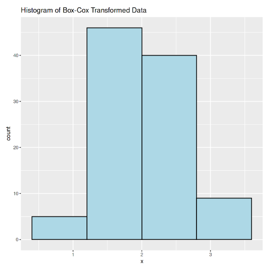
ggplot(data.frame(x = transformed_data), aes(x)) +
  geom_histogram(binwidth = 0.8, color = "black", fill = "lightblue") +
  ggtitle("Histogram of Box-Cox Transformed Data")

Output:

Histogram of non-normal positively skewed data

The rgamma() function generates a random sample of 100 values from a gamma distribution with shape parameter 6 and scale parameter 1. This produces a positively skewed distribution. The ggplot2 package is used to create a histogram of the data using geom_histogram(). The binwidth argument specifies the width of the bins in the histogram, while the color and fill arguments determine the color of the bars.

The BoxCoxTrans() function from the caret package is then used to perform a Box Cox transformation on the data. This function automatically finds the optimal lambda value for the transformation based on maximum likelihood estimation. The transformed data is stored in the transformed_data variable. Finally, a histogram of the transformed data is created using ggplot2 and plotted in a similar manner as the original histogram.

Histogram of positively skewed normal data

Negatively Skewed Data

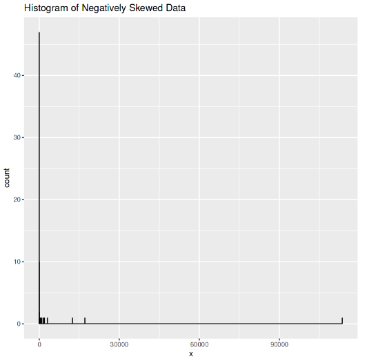
Negative Skewed data means when the tail of the left side of the distribution is longer than the tail on the right side. The mean and median will be less than the mode. Let us apply the Box Cox transformation to the positively skewed data.

In this example, we will generate a histogram of negatively skewed data and then performs a Box Cox transformation on the data using the caret package in R. The transformed data is then plotted as a histogram.

R

# load the libraries
library(caret)
library(ggplot2)

# define the dataset
set.seed(133)
data <- rlnorm(100, meanlog = 0, sdlog = 5)

# plot histogram of negatively skewed data
ggplot(data.frame(x = data), aes(x)) +
  geom_histogram(binwidth = 0.8, color = "black", fill = "lightblue") +
  ggtitle("Histogram of Negatively Skewed Data")

# boxcox transformation using caret package
bc_trans <- BoxCoxTrans(data)
transformed_data <- predict(bc_trans, data)

# plot histogram of transformed data
ggplot(data.frame(x = transformed_data), aes(x)) +
  geom_histogram(binwidth = 0.5, color = "black", fill = "lightblue") +
  ggtitle("Histogram of Box-Cox Transformed Data")

Output:

Histogram of negatively skewed data

The rlnorm() function is used to generate a random sample of 100 values from a lognormal distribution with a mean of 0 and a standard deviation of 5 on the log scale. The ggplot2 package is used to create a histogram of the data using geom_histogram(), with a binwidth of 0.8, and with the bars colored black and filled with light blue.

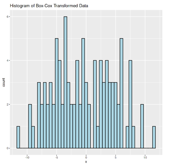
Histogram of negatively skewed normal data after Box Cox transformation

The BoxCoxTrans() function from the caret package is then used to perform a Box Cox transformation on the data. This function automatically finds the optimal lambda value for the transformation based on maximum likelihood estimation. The transformed data is stored in the transformed_data variable. Finally, a histogram of the transformed data is created using ggplot2 with a binwidth of 0.5 and plotted with the bars colored black and filled with light blue.